Is That Back-Test Result Good or Just Lucky?

by Michael R. Bryant

When developing trading strategies, most systematic traders understand that if you search long enough, you're bound to find something that looks great in back-testing. The question is whether those great results are from a great trading strategy or because the best looking strategy was the one that benefited the most from good luck. A well-known metaphor for this is a roomful of monkeys banging on typewriters. Given enough monkeys and enough time, one of the monkeys is likely to type the complete works of William Shakespeare just by random chance. That doesn't mean the monkey is the reincarnation of Shakespeare.

The same logic applies to developing trading strategies. When a trading strategy is chosen from among many different strategies or variations of strategies, good back-tested performance may be the result of good luck rather than good trading logic. A trader who knows the difference could save considerable time by avoiding further effort on a strategy that is inherently worthless and avoid the financial loss that would likely result if the strategy were traded live.

Whether great back-testing results are due mostly to random chance or to something more can be determined by applying a suitable test of statistical significance. The difficulty is in identifying the correct test statistic and in forming the corresponding sampling distribution. This article will present a method for calculating a valid significance test that takes advantage of the unique characteristics of the genetic programming approach to strategy development in which a large number of candidate strategies are considered during the development process.

The Basics of Significance Testing

Any effect we can measure that is subject to random variation can be represented by a statistical distribution. For example, a statistic that is normally distributed can be represented by its average and standard deviation. When this distribution is drawn from a sample of the entire population, the distribution is known as a sampling distribution. Characteristics of the sampling distribution will generally differ at least slightly from those of the population. The difference between the two is known as the sampling error.

A significance test is performed by assuming the so-called null hypothesis, which asserts that the measured effect occurs due to sampling error alone. If the null hypothesis is rejected, it's concluded that the measured effect is due to something more than just sampling error (i.e., it's significant). To determine whether the null hypothesis should be rejected, a significance or confidence level is chosen. For example, a significance level of 0.05 represents a confidence level of 95%. The so-called p-value is the probability of obtaining the measured statistic if the null hypothesis is true. The smaller the p-value the better. If the p-value is less than the significance level (e.g., p < 0.05), then the null hypothesis is rejected, and the test statistic is deemed to be statistically significant.

For a one-sided test, the significance level, such as 0.05, is the fraction of the area under the sampling distribution at one end of the curve. For example, if we're testing whether the net profit from a trading strategy is statistically significant, we would want the net profit from the strategy to be greater than 95% of the net profit values on the sampling distribution so that fewer than 5% of the points on the sampling distribution had net profits greater than the strategy under test. If that were the case, the trading strategy would have a p-value less than 0.05 and would therefore be considered statistically significant with 95% confidence.

How Does This Relate to Trading?

The key components of the significance test are the test statistic, the null hypothesis, and the sampling distribution. For evaluating trading strategies, each of these will depend on whether a single trading strategy is evaluated or multiple strategies are evaluated to select the best one. Let's first consider the case of evaluating a single trading strategy in isolation. It's assumed that the strategy was developed without evaluating different input values or combinations of trading logic. In this case, the test statistic can be any meaningful metric of strategy performance, such as net profit, risk-adjusted return, profit factor, or the like.

As an example, let's take the average trade as the test statistic. A suitable null hypothesis would be that the average trade is zero; i.e., that the trading strategy has no merit. The sampling distribution of the test statistic would be the distribution of the average trade. The p-value in this case can be determined from the Student's t distribution¹ and represents the probability of obtaining the strategy's average trade when it's actually zero (i.e., when the null hypothesis is true). If this probability is low enough, such as p < 0.05, then the null hypothesis would be rejected, and the average trade would be considered significant.

The preceding significance test is included in Adaptrade Builder as the "Significance" metric. In Builder, this metric is intended to be used as a measure of strategy quality. However, the Builder software generates and selects trading strategies based on a genetic programming process in which a potentially large number of trading strategies are evaluated before arriving at the final selection. As Aronson explains in detail,² the forgoing test of significance does not apply in this case. When multiple trading strategies are evaluated as alternatives and the best one is chosen, the test statistic, null hypothesis, and sampling distribution are all different than in the preceding example.

Data Mining Bias and the Test Statistic

When a trading strategy is developed by considering more than one rule, parameter value, or other aspect and choosing the best one, the performance results are inherently biased by the fact that of all the combinations considered, the one that generated the best result was chosen. Aronson explains and illustrates this effect in detail in his excellent book.² The resulting so-called data mining bias is a consequence of the fact that a trading strategy's results are due to a combination of randomness and merit. If multiple strategies are evaluated, the best one is likely to be the one for which the random component contributed heavily to the outcome. The component of randomness in the chosen strategy provides the data mining bias.

The data mining bias effectively shifts the mean of the sampling distribution to the right. In the example above, the sampling distribution of the average trade had a mean of zero, consistent with the null hypothesis. If we had chosen the strategy in question from among 1000 different strategies, the sampling distribution would have to take this feature of the search process into account. In general, to test the statistical significance of a strategy selected as the best strategy of a set of strategies, the sampling distribution has to be based on the test statistic that represents selecting the best strategy from a set of strategies. The test statistic for the example above in this case would not be the average trade but rather the maximum value of the average trade over the set of considered strategies. In other words, we want to know if the maximum value of the average trade over the set of considered strategies is statistically significant. Because the test statistic is based on the maximum over all strategies, the mean of the sampling distribution will be shifted to the right. This in turn will increase the threshold for significance as compared to the single-strategy test discussed above. So, by adopting this "best-of-N" statistic for significance testing, the effect of the data mining bias will be included in the sampling distribution and the resulting p-value will account for this effect.

Calculating the Sampling Distribution

Aronson presents a viable method for calculating the sampling distribution when the best-of-N statistic applies, as in data mining.² The Monte Carlo permutation method he discusses pairs trade positions with daily market price changes. The trade positions are randomized (selection without replacement) for each permutation. The null hypothesis is that the trading strategy is worthless, which is achieved by the random pairing of trade positions with market price changes. For each permutation, the performance of the randomly generated price-position series is evaluated for each considered strategy. The value of the metric for the best performing series is recorded as one point on the sampling distribution. The process is then repeated for as many permutations as desired to fill out the sampling distribution.

While the Monte Carlo method presented by Aronson benefits from computational simplicity, its reliance on daily (or bar-by-bar) positions (flat, long, short) makes it difficult to represent trading behavior accurately, such as when entering the bar at a specific price or if a trade enters and exits on the same bar. It also makes it difficult to properly include trading costs.

I propose an alternative approach here that takes advantage of the unique characteristics of the genetic programming process to strategy building. In Adaptrade Builder, the genetic programming process starts with an initial population of randomly generated strategies. The initial population is then evolved over some number of generations until the final strategy is selected. The key is that the algorithm is designed to generate strategies at random, which have no merit by design. As a result, the initial population offers a way to generate a sampling distribution.

The corresponding null hypothesis is that the strategy is no better than the best randomly generated strategy. As will be shown below, a randomly generated strategy is unprofitable on average. However, the best randomly generated strategy benefits from sampling error. Accordingly, if our strategy is no better than than the best randomly generated strategy, it's performance is likely due to sampling error alone. The alternative hypothesis is that the strategy has enough trading merit to improve the performance over what would be found if the strategy was no better than the best randomly generated strategy.

In Builder, the strategies are selected based on the so-called fitness. The appropriate test statistic for Builder is therefore the maximum fitness over all generated strategies. For statistical testing, we want to know if the strategy with the highest fitness over all generated strategies is statistically significant or if its results are due solely to sampling error.

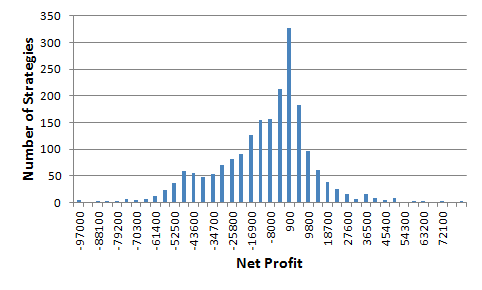
First, consider Fig. 1, below, which depicts the distribution of net profit from 2000 randomly generated strategies. As can be seen, the distribution supports the assumption that the randomly generated strategies have no trading merit. Nonetheless, due to sampling variability, the strategies range in profitability from -$102,438 to $71,858.

Figure 1. Distribution of the net profit of 2000 randomly generated trading strategies for the E-mini S&P 500 futures (daily bars, 13 years, trading costs of $15 per trade). The average net profit is -$12,340. The most profitable strategy has a net profit of $71,858.

To form the sampling distribution for the proposed significance test, the number of strategies generated during the build process in Builder is counted. This is equal to the total number of generations, including re-builds for which the process is re-started, multiplied by the number of strategies per generation. The number of strategies in the initial populations, including the initial populations for rebuilds, are then added to the total. For example, if there are 20 generations of a population of size 100 with no rebuilds, the total number of strategies is 2100.

If we call the total number of strategies N, each point of the sampling distribution is generated by creating N random strategies. All N strategies are evaluated using the same settings as during the build process, and the fittest strategy out of the N randomly generated strategies is selected. This creates one point of the sampling distribution. The process is then repeated for as many samples as desired. In the examples below, 500 samples were used to create each sampling distribution.

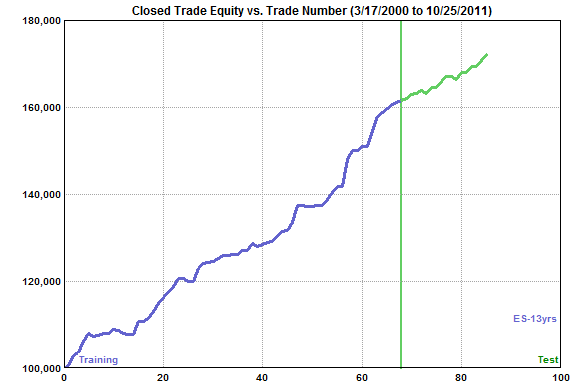
Example 1: A Positive Significance Result

To illustrate the proposed significance testing method, consider the equity curve shown below (Fig. 2) for a strategy generated by Adaptrade Builder for the E-mini S&P 500 on daily bars (3/17/2000 to 10/25/2011) with $15 per trade, and 1 contract per trade. A population size of 100 strategies was used. The build process consisted of a total of 63 generations, including 5 rebuilds, for a total of 6900 strategies.

 Figure 2. Equity curve for an E-mini S&P 500 strategy selected from 6900 total strategies.

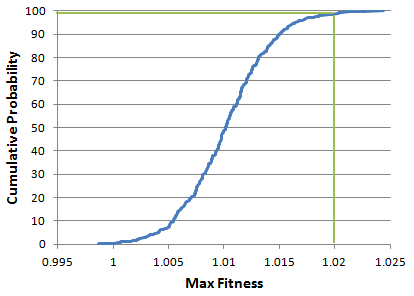
The cumulative sampling distribution for this strategy, generated according to the procedure given above, is shown below in Fig. 3.

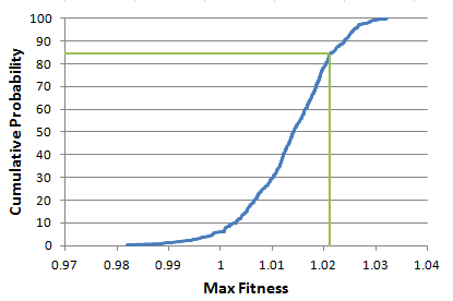
Figure 3. Cumulative sampling distribution for the maximum fitness for the strategy shown in Fig. 2. The strategy under test is identified by the green lines.

The fitness of the strategy depicted in Fig. 2 was 1.020. The location of this fitness value on the corresponding sampling distribution is shown by the green lines in Fig. 3. The fitness value of 1.020 corresponds to a cumulative probability of 98.7%, which is equivalent to a p-value of 0.013, implying that the strategy is statistically significant at the 0.05 level. Put another way, the probability of achieving a fitness value of 1.020 if the strategy is in fact no better than the best randomly generated strategy is only 1.3%.

Interestingly, this strategy has a small number of trades, which would generally work against it being statistically significant. However, its performance metrics are very good: profit factor of 16, almost even split of profits between long and short trades, high percentage of winning trades (76%), high win/loss ratio (4.9), and so on. Unfortunately, there were only two trades in the "validation" segment following the test segment shown above, so the validation results are not reliable. Nonetheless, both of those trades were profitable.

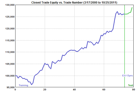
Example 2: A Negative Significance Result

The preceding example illustrated a strategy that was statistically significant according to the proposed procedure. This example will illustrate a strategy that fails the significance test even though its out-of-sample performance was positive. Consider the equity curve shown below in Fig. 4. This was based on the same settings as the prior strategy. The build process consisted of a total of 10 generations, with no rebuilds, for a total of 1100 strategies. Because there were no rebuilds, the test segment was not used in building the strategy. The results on that segment are therefore out-of-sample.

 Figure 4. Equity curve for an E-mini S&P 500 strategy selected from 1100 total strategies.

The cumulative sampling distribution for this strategy, generated according to the procedure given above, is shown below in Fig. 5.

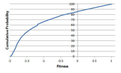
Figure 5. Cumulative sampling distribution for the maximum fitness for the strategy shown in Fig. 4. The strategy under test is identified by the green lines.

The fitness of the strategy depicted in Fig. 4 was 1.021.* The location of this fitness value on the corresponding sampling distribution is shown by the green lines in Fig. 5. The fitness value of 1.021 corresponds to a cumulative probability of 83%, which is insufficient to reject the null hypothesis at the 95% confidence level. The fitness is therefore not statistically significant at this confidence level.

Although the strategy appears that it might be viable based on its out-of-sample results, it is not statistically significant. Its apparent good performance is likely the result of random good luck.

Another Approach

There's another approach to the problem of evaluating significance when a trading strategy is selected from multiple candidates. It's based on the multiple testing correction to standard significance tests. The basic idea is to lower the significance level based on the number of tests. The most common correction is the Bonferroni method,³ which divides the significance level by the number of tests. For example, if 1100 strategies were evaluated, the significance level of 0.05 would be reduced to 0.05/1100 or 0.0000454. Obviously, this makes it much more difficult to detect significance. However, the sampling distribution used for detection is unadjusted for the data mining bias in this case.

As an example, consider the strategy in Fig. 2, above. This strategy was selected from 6900. The uncorrected significance level of 0.05 thus becomes 0.05/6900 or 0.0000072, which is equivalent to 99.9993% confidence. To detect this level of significance requires at least several hundred thousand samples. The test statistic in this case is just the fitness of a randomly generated strategy, and the sampling distribution consists of the distribution of this statistic computed from some large number of randomly generated strategies. To generate a suitable distribution, 500,000 randomly generated strategies were evaluated, and the fitness was recorded for each one, as shown below in Fig. 6.

Figure 6. Cumulative sampling distribution for the fitness for the strategy shown in Fig. 2.

Recall that the fitness of the strategy in Fig. 2 was 1.020. In Fig. 6, the maximum fitness in the sampling distribution is 1.0198. The p-value is therefore less than 1/500,000 or 0.000002 (99.9998%), which is less than the significance level of 0.0000072 (99.9993%). The null hypothesis can be rejected according to the Bonferroni test and the strategy declared significant.

This method agrees with the results of the prior method and does offer some computational savings. However, it's a more approximate method than directly computing the statistically correct sampling distribution. Harvey and Liu³ discuss and recommend other, related methods that offer refinements to Bonferroni.

Conclusions

Determining whether strategy results are due to a good strategy or just good luck is essential when strategies are developed using sophisticated discovery and search tools, such as Adaptrade Builder, which can generate and test thousands of strategies en route to the end result. This article discussed the nuances of statistical significance testing in this environment and how it differs from standard tests of significance. A method specifically suitable to the genetic programming approach of tools like Builder was proposed and illustrated. A simpler though less accurate method based on a correction to the standard significance test was also presented. Both approaches seem to generate suitable results.

The proposed method based on constructing the sampling distribution from randomly generated strategies has one drawback. It's very computationally intensive and therefore very time-consuming. With, for example, just 1100 strategies and 500 samples, a total of 550,000 randomly generated strategies need to be simulated, which can take several hours. The method proposed by Aronson based on Monte Carlo permutations of the equity changes is probably much more efficient, though it has the limitations noted previously.

The statistical significance tests presented in this article should be a valuable addition to a trader's toolbox of strategy testing methods. However, these methods are not meant to replace testing a strategy on data not used in the build process, including forward testing in real time. Rather, adding significance testing to one's current testing methods should increase the overall reliability of the strategy development process, reduce time spent on strategies that have little or no intrinsic value, and reduce the likelihood of trading something that is unlikely to be profitable.

Good luck with your trading.

Mike Bryant

Adaptrade Software

_____________________

* Fitness values are not comparable between different builds because the scaling factors are calculated at the beginning of each build. Fitness values can be compared between generations and between the calculation of the strategy and the generation of the sampling distribution because the scaling factors are fixed throughout these calculations.

This article appeared in the April 2015 issue of the Adaptrade Software newsletter.

HYPOTHETICAL OR SIMULATED PERFORMANCE RESULTS HAVE CERTAIN INHERENT LIMITATIONS. UNLIKE AN ACTUAL PERFORMANCE RECORD, SIMULATED RESULTS DO NOT REPRESENT ACTUAL TRADING. ALSO, SINCE THE TRADES HAVE NOT ACTUALLY BEEN EXECUTED, THE RESULTS MAY HAVE UNDER- OR OVER-COMPENSATED FOR THE IMPACT, IF ANY, OF CERTAIN MARKET FACTORS, SUCH AS LACK OF LIQUIDITY. SIMULATED TRADING PROGRAMS IN GENERAL ARE ALSO SUBJECT TO THE FACT THAT THEY ARE DESIGNED WITH THE BENEFIT OF HINDSIGHT. NO REPRESENTATION IS BEING MADE THAT ANY ACCOUNT WILL OR IS LIKELY TO ACHIEVE PROFITS OR LOSSES SIMILAR TO THOSE SHOWN.

If you'd like to be informed of new developments, news, and special offers from Adaptrade Software, please join our email list. Thank you.