Optimal Strategy Diversification

by Michael R. Bryant

Portfolio diversification is generally regarded as one of the few free lunches in trading and investing. Proper diversification increases risk adjusted returns by reducing the volatility of the portfolio. For traders, this generally means you can increase your position size for a given level of risk and thereby increase overall returns. A multi-market, multi-strategy approach is often touted by trading advisors as the gold standard of diversification. But that means you need multiple trading strategies that complement one another. How do you find these strategies? This article will demonstrate an approach for finding trading strategies that produces optimal portfolio diversification.

Common Approaches to Portfolio Diversification for Traders

Before getting to the main point of this article, let's consider how traders typically diversify portfolios. Oftentimes, a trading strategy will be applicable to multiple markets. In this case, diversification might consist of starting with a broad basket of different markets and choosing which ones to include and exclude from the portfolio. The resulting portfolio would be defined by the selected markets and the allocation to each one. A portfolio analysis tool that can simulate trading all selected markets together can be used to model each possible portfolio. The final selection would typically be the combination that maximizes a key portfolio performance metric, such as the risk-adjusted return, net portfolio profit, etc.

Sometimes, a single trading strategy may be applicable to multiple markets but only with different parameter values for each market. In this case, the optimal portfolio not only requires choosing the markets to trade and the allocation to each one but the strategy parameter values for each market.

The correlation coefficient can sometimes be used to help identify the markets that are minimally correlated and therefore more likely to trade well together. However, this tends to be an indirect measure. The correlation between the price series of two markets is not the same as the correlation between the equity curves generated by strategies applied to those markets. Ultimately, it's how the equity curves match up that determines diversification, not the market prices themselves.

Unfortunately, calculating the correlation coefficient between two equity curves does not always help. Any two reasonably good trading strategies will generate equity curves that slope upward over time, approximating a straight line (at least on a fixed-contract/share basis). That implies that the correlation coefficient between the two equity curves will be close to 1 for any two such curves, making it difficult to glean useful information from the correlation coefficient of the equity curves.*

Both of the preceding cases achieve diversification across markets for the same strategy. Another approach is to diversify across strategies for the same market. Here, multiple strategies can be applied to the same market to see how well the resulting portfolio performs. Either through trial-and-error or using a more systematic approach, such as optimization, the combination that maximizes the chosen performance metric(s) can be found. The optimal portfolio in this case would be specified in terms of the specific strategies selected for the given market and the allocation to each strategy.

Lastly, as suggested in the introduction, diversification across markets for the same strategy and across strategies for the same market can be combined. Some trading advisors reportedly use dozens of different market-system combinations to achieve their diversification goals. However, one can imagine a point of diminishing return where the added diversification from one more market system is not worth the added complexity and risk associated with managing a larger portfolio.

A More Direct Approach

The commonly used approaches to diversification for trading portfolios described above all have one thing in common. They all assume the process begins with a given set of trading strategies. This is hardly surprising since, typically, good trading strategies are difficult to develop. However, the ability to rapidly develop a trading strategy and custom-tailor its performance characteristics changes this calculus. This is exactly what genetic programming provides as a method of strategy development.

Consider the following scenario. You develop a short-only strategy to trade the E-mini S&P and are satisfied with its performance as a stand-alone strategy. Nonetheless, you later decide to add to your portfolio. It's logical to think that a long-only strategy for the same market might work well in combination with your existing short-only strategy.

Rather than developing a long-only strategy as a stand-alone strategy, you decide to use a genetic programming (GP) approach to develop a long-only strategy based on how well it works in combination with your existing short-only strategy. The metrics guiding the build process are based on the portfolio equity curve, such as the net portfolio equity and the correlation coefficient of the portfolio equity curve. As a result, the long-only strategy found through the GP process is the one that works best in combination with the short-only strategy to produce the best combined results. Since you're ultimately interested in the overall performance of your portfolio, this is a more direct approach than trying to find existing strategies and/or markets that just happen to work well together.

In other words, instead of selecting an existing strategy and hoping it helps diversify the portfolio, this approach develops a new strategy specifically to work well with the existing portfolio. For example, if the existing portfolio has a drop in equity at the end of last June, the new strategy will ideally be designed to have an equity run-up towards the end of June, resulting in an overall smoothing of the portfolio equity curve. This can be achieved by building strategies that maximize the linearity of the portfolio equity curve. The GP process will build the strategy in whatever way is necessary to produce the straightest and smoothest equity curve for the portfolio.

An Example of Building for Optimal Portfolio Performance

To illustrate this approach, consider the equity curve shown below in Fig. 1.

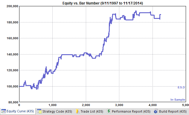
Figure 1. Bar-to-bar equity curve for a short-only E-mini S&P futures strategy.

This curve represents the bar-by-bar equity for a short-only strategy for daily bars of the E-mini S&P 500 futures developed using Adaptrade Builder.** Trading costs of $25 per trade were deducted, and position sizing of one contract per trade was employed. Mostly, default settings were used in Builder. For illustrative purposes, the build process for this strategy was intentionally abbreviated so that the resulting equity curve would not be particularly smooth. As a result, there are several notable flat spots in the equity curve: between approximately (1) bars 1 - 500, (2) bars 1200 - 2200, and (3) bars 2700 - 4200.

After the strategy was developed, the bar-by-bar equity curve, as shown above, was written out to a text file and added as an additional column of data in the price data file. The custom indicator feature of Builder was used to read in the equity curve values along with the price data. Using a prototype feature of Builder, the bar-to-bar equity changes calculated from this external equity curve were added to the equity values from each strategy being evaluated as part of the normal build process. The resulting equity curves therefore represented the combination of the equity curve shown above and the equity curve for the strategy being built; in other words, the portfolio equity curve. The performance metrics were then calculated based on the portfolio equity curve.

Using this prototype portfolio approach, a long-only strategy was built in Builder. The main build objectives were to maximize net profit and the correlation coefficient of the equity curve, which was chosen to generate a straight, smooth equity curve. Because the metrics were based on the combination of the long-only strategy's equity curve and the equity curve from the short-only strategy (Fig. 1), the build process was building a long-only strategy with the goal of achieving a smooth, straight portfolio equity curve. The result is shown below in Fig. 2.

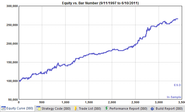
Figure 2. Bar-to-bar equity curve for a portfolio consisting of short-only and long-only E-mini S&P futures strategies, in-sample segment.

This figure represents the portfolio equity curve over the build (in-sample) segment for the combination of the long-only and short-only strategies. The fact that the curve is much smoother than the short-only strategy's curve suggests that the build process successfully found a long-only strategy that works well in combination with the short-only strategy. This can be understood better by looking at the equity curve of the long-only strategy by itself, as shown below in Fig. 3.

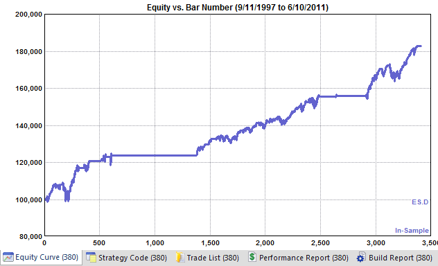
Figure 3. Bar-to-bar equity curve for a long-only E-mini S&P futures strategy designed to work well in combination with the strategy depicted in Fig. 1.

Similar to the equity curve in Fig. 1, this equity curve is not particularly smooth by itself. However, recall the three flat segments observed in Fig. 1. Comparing bar numbers between the two figures, it can be seen that for each of the flat segments in Fig. 1, the equity curve in Fig. 3 is rising. Conversely, there are two notable flag segments in Fig. 3: (1) bars 600 - 1400, and (2) bars 2500 - 2900. In Fig. 1, the equity curve for the short-only strategy shows rising equity for both of these segments. The build process was able to find a long-only strategy that almost perfectly complements the short-only strategy, rising where the short-only strategy is flat and staying flat where the short-only strategy rises.

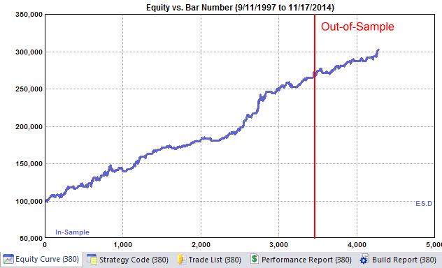
Finally, consider the out-of-sample performance for the combined short-only and long-only portfolio, as shown in Fig. 4, below. It's true that the short-only strategy included out-of-sample results, but, as can be seen in Fig. 1, those results were flat at best. Moreover, the long-only strategy was not built using the out-of-sample equity curve from the short-only strategy. Regardless, the out-of-sample results for the portfolio suggest that even out-of-sample, the long-only strategy complements the short-only strategy very well.

Figure 4. Bar-to-bar equity curve for a portfolio consisting of short-only and long-only E-mini S&P futures strategies, including out-of-sample segment.

Conclusions

This article examined portfolio diversification in terms of how trading strategies complement each other in a systematic trading portfolio. The point of view adopted here is that diversification is ultimately about how the portfolio performs, so that an optimally diversified portfolio of trading strategies is one in which the selected strategies generate the optimal portfolio results. It was shown that a genetic programming approach can be used to directly build a trading strategy to achieve the goal of optimal portfolio performance. Such a strategy can be said to be optimally diversified in that it generates the best risk-adjusted returns for the portfolio.

The example illustrated how the GP process can automatically find a strategy that precisely complements an existing strategy, with the strategy's equity rising when the other's is flat or falling, and vice-versa. The equity curve for the combination was much more linear than the equity curve for either strategy by itself, demonstrating substantial diversification with just two market systems.

Creating a diversified portfolio of systematic trading strategies doesn't have to be a trial-and-error process in which the final result is dependent on previously developed trading strategies that were not specifically designed to be traded together. Using a genetic programming process, each strategy can be custom-designed to complement the existing market systems in the portfolio, resulting in optimal portfolio diversification and therefore optimal portfolio results.

Good luck with your trading.

Mike Bryant

Adaptrade Software

____________

* As pointed out by one of my forum posters (https://groups.google.com/forum/?fromgroups#!topic/adaptrade-builder/BjUpgodjVVs), this problem can be addressed by using non-accumulated equity values, rather than the equity curve itself. This is equivalent to taking the correlation coefficient of the de-trended equity curves.

** The bar-by-bar equity curves shown in this article and the ability to build strategies based on an externally supplied equity curve are prototype features not yet available in current versions of Adaptrade Builder.

This article appeared in the November 2014 issue of the Adaptrade Software newsletter.

HYPOTHETICAL OR SIMULATED PERFORMANCE RESULTS HAVE CERTAIN INHERENT LIMITATIONS. UNLIKE AN ACTUAL PERFORMANCE RECORD, SIMULATED RESULTS DO NOT REPRESENT ACTUAL TRADING. ALSO, SINCE THE TRADES HAVE NOT ACTUALLY BEEN EXECUTED, THE RESULTS MAY HAVE UNDER- OR OVER-COMPENSATED FOR THE IMPACT, IF ANY, OF CERTAIN MARKET FACTORS, SUCH AS LACK OF LIQUIDITY. SIMULATED TRADING PROGRAMS IN GENERAL ARE ALSO SUBJECT TO THE FACT THAT THEY ARE DESIGNED WITH THE BENEFIT OF HINDSIGHT. NO REPRESENTATION IS BEING MADE THAT ANY ACCOUNT WILL OR IS LIKELY TO ACHIEVE PROFITS OR LOSSES SIMILAR TO THOSE SHOWN.

If you'd like to be informed of new developments, news, and special offers from Adaptrade Software, please join our email list. Thank you.