Adaptrade Software Newsletter Article

Optimization has had a role in trading strategy development for as long as I've been involved in trading — roughly thirty years now. Even among traders who claim to never optimize, their strategies often consist of indicators, parameter values, stop sizes, and other features that they've found through practical experience work best. That itself is a form of optimization. However, while the presence of optimization has been a constant for all that time, the methods of optimization have evolved.

In this article, I'll propose a relatively simple approach to optimization that runs counter to the prevailing pedagogy but which I believe may be preferable to more complicated methods that are currently taught. I'll first present a brief history of optimization in strategy development over the past thirty years from my personal perspective. I'll then argue that the lessons learned over that time make it feasible to use a comparatively simple optimization approach without incurring the drawbacks encountered in the past. I'll outline my proposed method and close with an example employing my trading strategy generator, Adaptrade Builder.

Trading Strategy Optimization Then and Now

When I first started developing trading strategies in the early 90's, optimization was primarily applied to existing trading strategies to optimize their parameter values — indicator look-back lengths, oscillator levels, stop sizes, and so on. Optimization was a controversial topic, and the statistical concept of over-fitting was often described inaccurately as "curve-fitting".^{1, 2} In many cases, optimizations were performed on all available data, without leaving aside data for out-of-sample testing. Many of the best practices strategy developers and traders utilize today didn't exist at that time.

It's now widely understood that it's not curve-fitting per se that's problematic but over-fitting. Curve-fitting is just another name for optimization. Over-fitting, on the other hand, occurs when the optimization process fits the strategy to the market's noise, rather than just the signal. The signal is the part of the market that contains predictive information, whereas the noise is random. If the strategy fits too much of the noise, it may look good in hindsight but have little predictive power.

Thirty years ago when computers were less powerful and market data less plentiful — intraday data was expensive and harder to come by — an optimized strategy may have had no more than 30 trades over five years of daily bars — not enough data in most cases to avoid over-fitting. To make matters worse, optimizations were often performed by maximizing a single metric, such as net profit, without considering metrics related to strategy robustness. It's hardly surprising that over-fitting was common and that optimization got a bad reputation as a result.

To address the likelihood of optimized strategies failing post-optimization, an early recommendation was simply to perform out-of-sample (OOS) testing.^{2, 3, 4} In other words, set aside a segment of data not used in the optimization to provide an unbiased measure of strategy performance following the optimization. However, a common problem with this approach is what happens when the OOS test fails. Do you make a change to your strategy and test again on the same OOS segment? If you run multiple tests like that until the OOS results look good, you run the risk of introducing so-called selection bias — you select the strategy that happens to perform best on the OOS segment.⁵

Another early suggestion to improve optimization results was looking at the robustness of the optimal parameter values. It was recognized that the optimal parameter set, even if it's not over-fit, may change in the future; i.e., the best parameter values going forward might be different than the ones that were optimal in the past. Schwager recommended using average parameter sets³ to address this problem while Stridsman suggested "altering the inputs"⁴ to assess the robustness of the optimized values. In optimization theory, this is referred to as sensitivity analysis.⁶ For example, suppose you're optimizing the look-back length of an indicator by maximizing net profit, and the optimal look-back length is 13 (i.e., the maximum net profit occurs at a look-back length of 13). You would also consider the net profit at indicator lengths of, say, 11 to 15. If the net profit was acceptable at those lengths as well, then 13 would be accepted as the optimal result. On the other hand, if the net profit dropped off sharply at values other than 13, then you would look for other look-back lengths around which the net profit was more stable.

One of the best known and most rigorous methods to improve trading strategy optimization and avoid over-fitting is walk-forward optimization, introduced by Robert Pardo in his 1992 book, Design, Testing, and Optimization of Trading Systems.⁷ The basic idea of walk-forward optimization is straightforward: segment the data into consecutive time periods, optimize over the first segment, test forward, move to the next segment, and repeat. Because each forward segment is not used in the preceding optimization, the results on those segments provide an unbiased measure of the optimized strategy's performance; i.e., the walk-forward segments are out-of-sample. And because there are multiple segments, there's no need to repeat the optimization over the in-sample (optimization) segments, so you avoid the selection bias problem.

Walk-forward optimization can be thought of two ways. First, as mentioned above, the OOS segments provide an unbiased measure of strategy performance. Second, it can be viewed as a test of the optimization method itself. In practice, it's helpful to know the likelihood of profitable results if you optimize your strategy over data up through the current date. If you perform a walk-forward optimization using, say, 15 OOS periods, and 12 of them are profitable, you can have some confidence that roughly 80% of the time, your results will be profitable going forward following the last optimization. Conversely, if none or very few of the OOS segments show profitable results, it suggests there's a problem with the optimization.

Another trend that influenced optimization methods for trading was the rise of machine learning methods starting in the mid 2000s. Because machine learning involves fitting models to data, the machine learning community popularized a number of techniques to minimize the risk of over-fitting. While a broad discussion of these methods is beyond the scope of this article, some of them include so-called regularization techniques, such as adding a penalty for complexity, cross-validation, and early stopping. Also, machine learning practitioners often use a three-segment division of the data — training, test, and validation — in which the optimization is performed over the training segment, the next segment (called either test or validation) is used to monitor the training, and the final segment (called either validation or test) is set aside for an unbiased estimate of performance.⁵ The third segment addresses the problem of selection bias discussed above.

Other methods for avoiding over-fitting in optimization have since been developed either specifically for trading or for machine learning and artificial intelligence. Many of these methods can be found in modern trading software, such as in Adaptrade Builder. For example, adding "noise" to the input data helps prevent the optimization from over-fitting specific data features that may not contribute to generalization, such as a price spike that is unlikely to repeat. Builder includes special rules that monitor the test segment to detect over-fitting and can either restart or terminate the optimization if over-fitting is detected. More sophisticated optimization metrics also help. For example, rather than simply maximizing net profit, Builder allows the user to set conditions for metrics that relate to the quality and robustness of the trading strategy, such as the statistical significance of the average trade, entry and exit efficiency, and maximum adverse excursion, among others.

No Approach is Perfect

While modern optimization methods represent a significant improvement over approaches commonly employed 30 years ago, there are still challenges. For example, not all machine learning optimization methods are applicable to trading due to differences in the kind of data used. In machine learning, the data are typically independent. For example, in training a neural network to learn to recognize images, the images used as training data are generally unrelated to each other and can be presented to the model in any order. Market data, on the other hand, have a time relationship with each other. This implies that cross-validation methods that randomly segment the data would not work for trading strategy optimization because they would disrupt any sequential patterns in the price data that might be important.

Another time-related complication for trading strategy optimization is that market data tend to be non-stationary.^{8, 9} In other words, the statistical properties of the data change over time. This is why most trading strategies tend to fail eventually. Non-stationary markets also complicate optimization because you ideally want to optimize over the most recent data so that the results will reflect current market dynamics. If you optimize over data that's too old, the market might have changed by the time you start trading. But if you optimize up through the current date, there won't be any data available for OOS testing.

This conflict between reserving data for OOS testing and using the most recent data available can be resolved to some extent by using walk-forward optimization. In that case, you have several OOS periods by which to judge the effectiveness of the optimization process. The final optimization before starting to trade the strategy can be performed on the most recent data. However, walk-forward optimization has drawbacks as well. In particular, by dividing the training data into multiple segments, there may not be enough trades to get reliable results in each segment.

Another difficulty with walk-forward optimization is the computational complexity: multiple segments means multiple optimizations. If each optimization is time-consuming, performing the entire walk-forward optimization can be prohibitive. While this is not usually a concern when optimizing the inputs to a trading strategy, it can be problematic for trading strategy generators, such as Adaptrade Builder, which optimize the design of the entire strategy — entry and exit rules, trading orders, parameter values, even position sizing. In the example I'll present below, a robust optimization over a single segment took about 24 hours. If I had used the same amount of training data for each of 10 segments, it would have taken about two weeks to perform a walk-forward optimization. Moreover, a walk-forward optimization using a strategy generator would build a different trading strategy for each segment, making it difficult to draw conclusions about performance from the OOS segments since you'd be comparing the results from different strategies.

Lessons Learned

If walk-forward optimization is not always practical, what's the alternative? Fortunately, several lessons can be gleaned from the past to provide some guidance. First, the causes of post-optimization failure are much better understood now. Aronson discussed the statistics of over-fitting in detail in terms of the data mining bias.¹⁰ Data mining is essentially another word for optimization in that it typically consists of comparing different solutions and selecting the best one. I discussed the sampling distribution and significant testing in a newsletter article as a way of understanding the data mining bias. Masters⁵ refers to the data mining bias as a combination of training bias and selection bias. However you describe it, it results from the selection process of optimization applied to candidate solutions that benefit from randomness. Choosing the best solution when some — perhaps many — of the solutions benefit from random good luck means there will likely be a positive bias to the chosen solution. If this bias is too large, the results are said to be over-fit.

While you can test the results to see if the solution is over-fit, it's also possible to minimize the chances of getting an over-fit solution in the first place. One way to do this is by making sure each candidate solution has a large number of trades. With more trades, it's less likely that the results could be due to chance. Similarly, it's generally the case that you get what you ask for — the out-of-sample results will tend to reflect the training objectives — so it's better to specify metrics that represent robust results, rather than using a single metric like net profit. For example, specifying optimization requirements for entry and exit efficiency, maximum adverse excursion (intra-trade drawdown), profit factor, and percentage of wins makes it more likely that the resulting strategies will display those desired characteristics out-of-sample.

Aronson also pointed out that, in general, data mining (and hence optimization), works: selecting the best solution from a large number of candidate solutions is better than choosing a solution at random.¹¹ It's also true that examining a larger number of solutions is better than selecting from fewer. The only caveat is that the sample size (e.g., number of trades) used to calculate the metrics needs to be large enough. The implication for a tool like Adaptrade Builder is that you will generally be better off letting it run for more generations, rather than fewer. While this would seem to contradict the purported benefits of so-called early stopping, letting the optimization run longer works as long as the solution is not being over-fit whereas early stopping can minimize over-fitting in cases where it would otherwise occur. In other words, letting the optimization run longer does not necessarily lead to over-fitting, but if over-fitting is occurring, stopping the optimization early may help.

The other cause of post-optimization failure is non-stationary market conditions. There are several ways to address changing market conditions, each with its pros and cons. The first possibility is to optimize over a longer series of price data that contains a variety of market conditions (e.g., both bull and bear markets, high and low volatility). The rationale is that the resulting strategies will be more likely to tolerate changing conditions in the future because they will have seen more kinds of conditions during training. The risk with this approach is that the strategy will be tailored to data and market conditions that are irrelevant — that the market has changed and will never repeat the patterns contained in the older data.

A second way to combat non-stationary markets is to monitor the strategy and stop trading it when its performance drops below its long-term average. I wrote an article many years ago for Stocks & Commodities magazine about so-called money management indicators that can be used for this purpose. The indicators themselves are still available on my web site in EasyLanguage format. The problem with this approach is that by the time you recognize that the strategy is no longer working, you have already lost money.

A more reliable approach is to systematically develop new strategies on a regular basis using the latest market data. With this approach, it's better to drop the old data when you add the most recent data in order to avoid biasing the strategies to the older data. If you trade a portfolio of strategies, you can then add the new strategy to your portfolio, dropping the worst performing strategy. If you trade a single strategy, you can simply replace it with the new strategy, hopefully before the old one has become unprofitable. The only real drawback of this approach is that you risk replacing a good strategy with a lesser one.

An Optimization Recipe for Strategy Building

Based on the discussion above, here is my recipe for employing optimization when building trading strategies using a strategy building tool such as Adaptrade Builder. You could also use this approach when optimizing the parameters of an existing trading strategy, although, as noted above, walk-forward optimization can also be effective in that simpler case.

1. Set the training/test/validation intervals to 100% training (i.e., no test or validation segments).
2. Set aside roughly 20% of the data for post-build validation. Don't use this data until the final optimization is complete.
3. Use enough data to get at least 300 trades while building.
4. Apply stress testing with Monte Carlo analysis using a small number of Monte Carlo samples, such as 5 - 10.
5. Use so-called quality metrics, as I discussed in a previous article and as illustrated in the exmaple below. Add complexity as an objective with a small weight to bias the solution towards simpler strategies.
6. Let the build process run for approximately 500 generations.
7. Dividing the population into several sub-populations with mixing every 20 - 100 generations may help maintain diversity.

The key to this approach is to not use the validation data until the very end. You can make as many adjustments to the metrics and other build settings based on the training data as you like. In fact, it's probably essential to perform multiple preliminary builds until you're confident your metrics are giving you what you want. When the builds on the training data look like they're going well, you can then let it run for the full 500 generations.

At the end of the build process, you should confirm that the results are what you wanted. Check the top strategy to make sure the number of trades is high enough, the equity curve looks good, the metric conditions are met or are close enough, and so on. If not everything meets your requirements, then make adjustments and repeat the build. If you did a sufficient number of preliminary builds, repeating the build should not be necessary. Once everything looks good, then (and only then) can you set the evaluation range to encompass the validation data and run an evaluation (back-test) on all the data. This will give you the out-of-sample results to validate the optimization.

If the out-of-sample results look good, then you can move the date range to include the validation segment so that the next optimization will include the most recent data up through the current date. In this case, it's recommended that you also move up the starting date to exclude the earlier data so that the number of bars of data remains the same. With the optimization results on the most recent data, you're ready to either validate in real time tracking or real time trading.

What happens if the out-of-sample evaluation fails? This suggests either over-fitting or non-stationarity. In this case, you can move the training date range back so that the validation/OOS segment overlaps the end of the previous training data — like walk-forward optimization but in reverse. This will give you another OOS period, which can help you to better understand the problem. If this OOS period also fails, it may be over-fitting, in which case the solution may be to start over with a longer training period. If the second OOS period is valid, then the problem may be non-stationarity. This problem is harder to address but may be resolved by moving to a different (preferably larger) bar size, increasing the length of the training period, or perhaps changing symbols.

An Example

To illustrate the points discussed above, I ran an example build in Adaptrade Builder on 15-minute bars of the E-mini S&P 500 futures, day session only (Fig. 1).

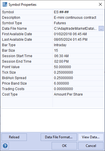
Figure 1. Symbol properties for the E-mini symbol used in the build example.

The training segment was set to 100% of the date range minus one year, which was set aside for the out-of-sample testing. The trading costs were set to $5 per round turn, and the position sizing was set to one contract per trade. The build metrics are shown below. These were arrived at by first adding the complexity metric to the set of default build objectives then adding the quality metrics for entry and exit efficiency, DoF ratio, profit factor, Kelly f, maximum adverse excursion (MAE), correlation coefficient, and trade significance. Based on several short trial runs, I then added conditions for the average trade size and the maximum bars in trades to obtain the results on the training data that I wanted.

                            Maximize Net Profit, weight 1.000
                            Maximize Corr Coeff, weight 1.000
                            Maximize Trade Sig, weight 1.000
                            Minimize Complexity, weight 0.100

                            Max Bars <=  100 (Train)
                            Ave Trade between  $100.00 and $300.00 (Train)
                            Ave Exit Efficiency >=  60.00% (Train)
                            Ave Entry Efficiency >=  60.00% (Train)
                            DoF Ratio between  1.000 and 3.000 (Train)
                            Prof Fact >=  2.000 (Train)
                            Kelly f >=  20.00% (Train)
                            Max MAE (%) <=  5% (Train)
                            Corr Coeff >=  0.9500 (Train)
                            Trade Sig >=  95.00% (Train)
                            

I selected Monte Carlo stress testing with five samples at 95% confidence using the default settings for the stress testing methods. I used 500 generations with a population size of 500 and two subpopulations mixed every 20 generations. Most of the other settings were left at their default values, which can be obtained from the project file.

The project file and code file in text file format are provided below. The project file can be opened in Adaptrade Builder 4.7.1 or later. The code file is in EasyLanguage (TradeStation and MultiCharts).

Example Downloads: Project File (.gpstrat); Code File (.txt)

The build progress curve for the example is shown below is Fig. 2. Although the fitness appears to flatten out after as few as 40 generations, the fitness shown on the curve is the average fitness for the population. The fitness of the top (fittest) strategies in the population continued to improve even after several hundred generations.

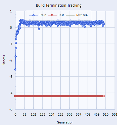
Figure 2. Build progress curve, showing how the fitness on the training segment evolved over 500 generations. The curve represents the average fitness over all members of the population.

The equity curves for the top strategy in the population are shown below in Figs. 3 and 4. The plot in Fig. 3 shows the Monte Carlo curves over the training segment. In Fig. 4, the curve includes the out-of-sample results on the one-year segment set aside prior to the optimization.

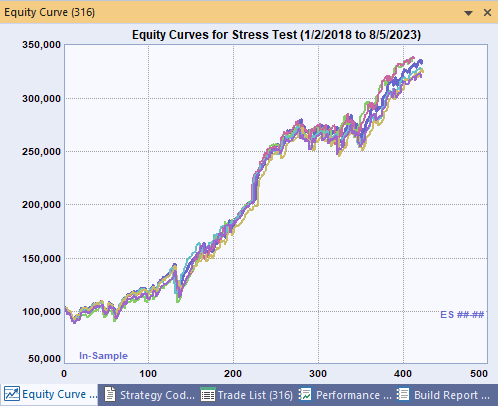
Figure 3. Equity curves including the stress testing (Monte Carlo) curves on the training segment.

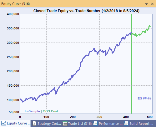
Figure 4. Equity curve including both the training and out-of-sample segments.

The results on the OOS segment are similar to those on the in-sample segment, supporting the proposed approach. If I were intending to trade the strategy live, the next steps would be to move the starting and ending dates for the training segment forward one year (or, more precisely, up to the current date) and repeat the optimization. Finally, I would probably track the strategy in real time for at least a few trades to make sure there were no surprises before committing real money.

One aspect of this approach that is not reflected in the figures shown above is how long it can take. The full optimization encompassing 500 generations took just over 24 hours. Other than the large number of generations, the reason it took so long is that the build time is a linear function of the number of Monte Carlo samples, and, since the results are already processed in parallel, there's no way to avoid that linear scaling relationship. This is one of the reasons why walk-forward optimization is not ideal for strategy building tools, such as Adaptrade Builder: to repeat the optimization over the multiple periods of a walk-forward optimization would require an unreasonably long time.

Summary and Discussion

Trading strategy optimization is not nearly as problematic today as it was several decades ago when systematic trading was still a fairly new idea (at least to the retail trading community). And while the advent of trading strategy generators, such as Adaptrade Builder, complicates the optimization problem, the better understanding we now have of how optimization works more than compensates for the increased burden imposed by the requirements of strategy generators.

The optimization approach I proposed in this article incorporates a variety of techniques to avoid over-fitting: regularization (low complexity), build metrics related to strategy quality, stress testing (noise injection), a high number of trades (sufficient data), long build times, and out-of-sample validation. In effect, the combination of these different techniques is a trade-off against the fact that only one OOS period is examined. For the same build time, an alternative would be to use a simpler approach (e.g., no stress testing, less data) in a walk-forward optimization, resulting in more OOS segments. The downside would be that each optimization would be less robust and less reliable. I'm arguing that it may be better to perform one robust and reliable optimization than several that we may not be able to trust.

One limitation of the proposed approach is that with only one OOS segment, it's difficult to estimate the true performance of the strategy. The OOS segment can be used for this purpose, but since there is only one such segment, the estimate may be less reliable than if a walk-forward approach was used. This may or may not make a difference in practice, depending on whether you intend to use the back-test results to set allocations, position sizing, and so on. Nonetheless, provided the OOS segment was not reused, as it was not in the example presented above, it still offers an unbiased estimate of performance.

Trading strategy optimization is an inescapble aspect of trading strategy development for most traders. Accordingly, understanding how it works and, more importantly, how it can fail, is critical for trading success. While walk-forward optimization may be the gold standard for optimizing the inputs or parameters for an existing trading strategy, it's not always practical for generating entire trading strategies from scratch. In those cases, the roboust optimization approach I've outlined here may be a suitable alternative. Finally, as with any strategy development, whether it involves optimization or not, real-time tracking is always recommended before going live.

References

1. Babcock, B. Jr. The Business One Irwin Guide to Trading Systems, Business One Irwin, Homewood, IL, 1989, p. 44-52, 73-92.
2. LeBeau, C., Lucas, D. W. Technical Traders Guide to Computer Analysis of the Futures Market, McGraw-Hill, New York, 1992, p. 157-64.
3. Schwager, J. D. Schwager on Futures. Technical Analysis, John Wiley & Sons, Inc., New York, 1996, p. 695.
4. Stridsman, T. Trading Systems that Work, McGraw-Hill, New York, 2001, p. 331-7.
5. Masters, T. Assessing and Improving Prediction and Classification, Timothy Masters, 2013, p. 24-6. ISBN 978-1484137451.
6. Gill, P. E., Murray, W., Wright, M. H. Practical Optimization, Academic Press, Inc., Orlando, FL, 1981, p. 320-23.
7. Pardo, R. Design, Testing, and Optimization of Trading Systems, John Wiley & Sons, Inc., New York, 1992.
8. Sherry, C. J., Sherry, J. W. The Mathematics of Technical Analysis, ToExcel, San Jose, 2000, p. 9-83.
9. Bandy, H. B. Quantitative Technical Analysis, Blue Owl Press, Inc., Eugene, OR, 2015, p. 193-4.
10. Aronson, D. Evidence-Based Technical Analysis, John Wiley & Sons, Inc., New Jersey, 2007, p. 255-330.
11. Ibid., p. 309-11.

Good luck with your trading.

Mike Bryant
Adaptrade Software