Better
Optimization in TradeStation, Part 2
In the
November 2004 issue,
I presented a method for optimizing a trading system in TradeStation using a
custom objective function written in TradeStation's EasyLanguage scripting
language. The purpose of the EasyLanguage function, called EqtyCorr, was to make
it possible to find system parameter values that produce a relatively linear
equity curve with good net profitability. Trading systems with linear
(straight-line) equity curves have uniform profitability over different time
periods, which should make them more likely to perform well in the future
compared to systems that are more tailored to specific market conditions. In
this month's newsletter, I present an new objective function that has certain
advantages over the method previously presented.
Asking a trading system to
perform equally well in all time periods is a fairly arbitrary request given
that the markets themselves are anything but uniform. It probably makes more
sense to ask what the potential profit is over a given period and then ask the
system to perform as close to that potential as possible. This kind of thinking
led me to something I refer to as the ideal equity curve optimization method.
The basic idea is not new. In
his book "Design, Testing, and Optimization of Trading Systems" (John Wiley
& Sons, Inc., New York, 1992, pp. 74-75), Robert Pardo describes an
optimization method based on the "perfect profit," which he defines as the sum
of the absolute price differences. A trading system that generated perfect
profit would buy the close if the next day was going to close higher and sell
the close if the next day was going to be lower. Obviously, no such system is
possible, but the equity curve generated by this hypothetical system represents
the potential profit in the market. To use the perfect profit in system
optimization, Pardo maximized the correlation coefficient between the equity
curve represented by the perfect profit and the equity curve of the trading
system. The optimal system parameter values were those that resulted in the
equity curve closest to the perfect profit.
Rather than use the sum of the
absolute price differences to generate a "perfect" equity curve, my thought was
to identify a set of "ideal turning points" on a chart and use those turning
points to generate an ideal equity curve as if we were trading a
stop-and-reverse system through those points. By changing how the turning
points are chosen, the number of "trades" from this ideal system could be
adjusted to better match the number of trades from the trading system being
optimized. The ideal system would presumably represent the profit potential of
the actual trading system better if the ideal system generated about
the same number of trades as the actual system.

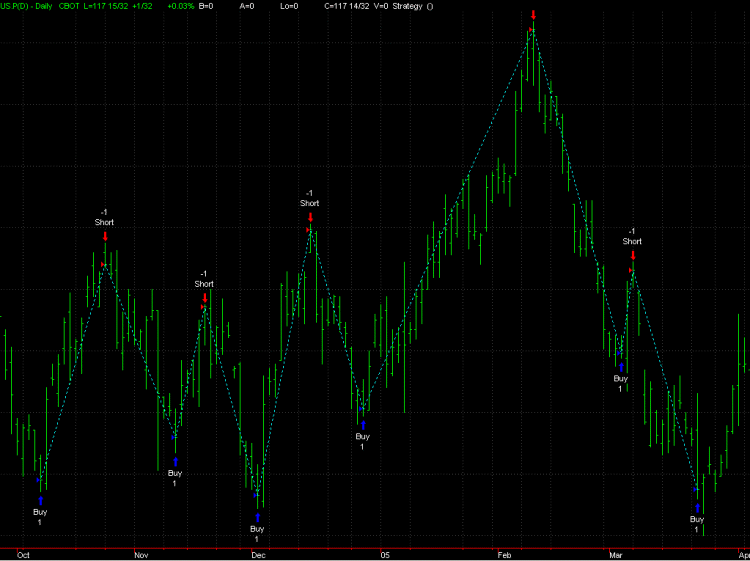
Figure 1. Ideal
turning points in T-Bond futures, as identified by
function IdealEqtyOpt5. The turning points are used to define a
hypothetical, ideal trading system that represents the profit potential in the
market.
Fig. 1
illustrates what I mean by "ideal turning points." The ideal turning points are
marked with buy and sell signals from a hypothetical system that reverses from
long to short and short to long at the turning points. How frequently the
reversals are triggered will depend on how big a market move it takes to reverse
the trend. In the function IdealEqtyOpt5, shown below in Fig. 2, the size of the
move needed to reverse the trend can be specified either in terms of
points or as a fraction of the n-day average true range. Once it has been
determined that the trend has reversed, the ideal turning point is located. When
the trend reverses from short to long, the turning point is the lowest close
since being short. When the trend reverses from long to short, the turning point
is the highest close since being long.
As an aside, the
ideal "trades" formed by the turning points might make a good training set of
trades for a neural network-based system. Rather than scanning a chart manually
to come up with trades to feed into the neural network, the method described
here could be used to automatically find the training set.
The
IdealEqtyOpt5 function keeps track of the equity from both the ideal
system and the actual trading system. The equity curve for the ideal system
is based on reversing from long to short at the high reversal points and from
short to long at the low reversal points. As with Pardo's perfect profit, a
system based on these ideal turning points is not possible in practice, but it
provides a measure of the potential profit in the market. On the last bar of the
chart, the function calculates the correlation coefficient of the ideal equity
and the equity from the trading system. The correlation coefficient and system
parameter values are appended to a user-specified text file for later
analysis.
To use the IdealEqtyOpt5
function to optimize a trading system, the same approach is used as described
for the EqtyCorr function presented previously. First, the function call is
added to the end of the trading system code, then the system is
optimized using TradeStation's optimization feature to iterate over all
combinations of the system's parameters. For each combination of parameter
values, the IdealEqtyOpt5 function will write one line to the text file
specified by the input parameter FName. As noted above, each line in the text
file will contain the correlation coefficient and the system parameter values.
After the optimization is complete, the lines in the text file can be sorted by
the value of the first column -- the correlation coefficient -- to find the
parameter values that maximize the correlation coefficient.
{
Function IdealEqtyOpt5
Calculate an
objective function based on the correlation
between the equity curve
generated by a trading system and the
"ideal" equity curve. The ideal
equity curve is the equity curve
generated by a stop and reverse
system that reverses at perfect
reversal
points.
The objective function value and system input
parameter values
are appended to a text file for later
analysis.
Copyright 2005 Breakout Futures
www.BreakoutFutures.com
}
input: Param1
(NumericSimple), { system parameter 1
}
Param2 (NumericSimple), { system
parameter 2 }
Param3 (NumericSimple), { system
parameter 3 }
Param4 (NumericSimple), { system
parameter 4 }
Param5 (NumericSimple), { system
parameter 5 }
Param6 (NumericSimple), { system
parameter 6 }
Param7 (NumericSimple), { system
parameter 7 }
Param8 (NumericSimple), { system
parameter 8 }
Param9 (NumericSimple), { system
parameter 9 }
Param10 (NumericSimple), { system
parameter 10 }
RevPts (NumericSimple), { points
to reverse }
RevFr (NumericSimple), {
fraction of ATR to reverse }
NRev
(NumericSimple), { length of ATR
}
RevType
(NumericSimple), { 0 = pts; 1 = ATR
}
FName
(StringSimple), { file name to write results to
}
PrintLog
(TrueFalse), { flag for writing to
print log }
WriteOpt
(TrueFalse); { True -> write
optimization; false -> write equity}
Var: LowC
(0), { lowest close
}
HighC
(0), { highest close
}
TrDir
(0), { direction of ideal trade
}
RevSz
(0), { points needed to reverse }
HighBar
(0), { number of bar with highest close
}
LowBar
(0), { number of bar with lowest close
}
ibar
(0), { bar counter
}
XVal
(0), { value of x, system equity
}
YVal
(0), { value of y, ideal equity
}
SumXY
(0), { sum of X * Y
}
SumX
(0), { sum of X
}
SumY
(0), { sum of Y
}
SumXX
(0), { sum of X * X
}
SumYY
(0), { sum of Y * Y
}
CCNum
(0), { numerator of correlation coefficient
}
CCDen
(0), { denominator of correlation coefficient
}
CorrCoef
(0), { correlation coefficient
}
ObjectFn
(0), { objective function
}
TotalEqty (0),
{ open plus closed trade equity }
ii (0), { loop
counter }
NBars
(0), { number of bars
}
NTrSys
(0), { number of system trades
}
NTrIdeal
(0), { number of ideal "trades"
}
StrOut
("");
Array: EqtySys[5000](0), { equity at
each bar, system trades }
EqtyIdeal[5000](0), { equity at each bar, ideal trades
}
TrSys[1000](0), { equity at end of
system trades }
DatesSys[1000](0), { dates of system trades
}
TrIdeal[1000](0), { equity at end of ideal trades
}
DatesIdeal[1000](0);
{ dates of ideal trades }
If BarNumber = 1 then Begin
If
Close > Close[1] then
TrDir =
1
Else
TrDir =
-1;
HighC = Close;
HighBar =
BarNumber;
LowC = Close;
LowBar =
BarNumber;
DatesSys[0] =
DateToJulian(date);
DatesIdeal[0] =
DateToJulian(date);
End;
If RevType = 0 then
RevSz =
RevPts
Else
RevSz = RevFr * average(TrueRange,
NRev);
If Close > HighC then Begin
HighC = Close;
HighBar =
BarNumber;
End;
If Close < LowC then
Begin
LowC = Close;
LowBar =
BarNumber;
End;
{ Reverse ideal trade from long to short }
If
TrDir = 1 and HighC - Close >= RevSz then Begin
TrDir =
-1;
NTrIdeal = NTrIdeal + 1;
If
PrintLog then
Print("Date: ",
date[BarNumber - HighBar]:0:0, " Time: ", time[BarNumber -
LowBar]:0:0,
" Close = ", HighC:0:4, " Direction: ", TrDir);
LowC =
Lowest(Close, BarNumber - HighBar + 1);
LowBar = BarNumber
- LowestBar(Close, BarNumber - HighBar + 1);
{ Adjust previous equity values from
reversal point to current bar }
For ii = ibar - (BarNumber
- HighBar - 1) to ibar - 1 begin
EqtyIdeal[ii] = EqtyIdeal[ii - 1] + (Close[ibar - ii + 1] - Close[ibar - ii]) *
BigPointValue;
End;
{ Record equity value and date for ideal
trade }
TrIdeal[NTrIdeal] = EqtyIdeal[ibar - (BarNumber -
HighBar)];
DatesIdeal[NTrIdeal] =
DateToJulian(date[BarNumber - HighBar]);
End;
{ Reverse ideal trade from short to long }
If
TrDir = -1 and Close - LowC >= RevSz then Begin
TrDir =
1;
NTrIdeal = NTrIdeal + 1;
If PrintLog then
Print("Date: ",
date[BarNumber - LowBar]:0:0, " Time: ", time[BarNumber - LowBar]:0:0,
"
Close = ", LowC:0:4, " Direction: ", TrDir);
HighC =
Highest(Close, BarNumber - LowBar + 1);
HighBar =
BarNumber - HighestBar(Close, BarNumber - LowBar + 1);
{ Adjust previous equity values from
reversal point to current bar }
For ii = ibar - (BarNumber
- LowBar - 1) to ibar - 1 begin
EqtyIdeal[ii] = EqtyIdeal[ii - 1] + (Close[ibar - ii] - Close[ibar - ii + 1]) *
BigPointValue;
End;
{ Record equity value and date for ideal
trade }
TrIdeal[NTrIdeal] = EqtyIdeal[ibar - (BarNumber -
LowBar)];
DatesIdeal[NTrIdeal] =
DateToJulian(date[BarNumber - LowBar]);
End;
{
Keep track of equity curve of trading system }
TotalEqty = NetProfit +
OpenPositionProfit;
If ibar < 5000 then
EqtySys[ibar] = TotalEqty;
{ Record equity value and date for system trade
}
If TotalTrades > NTrSys then Begin
NTrSys =
NTrSys + 1;
TrSys[NTrSys] =
NetProfit;
DatesSys[NTrSys] =
DateToJulian(date);
End;
{ Keep track of equity curve from ideal trades
}
If ibar > 0 and ibar < 5000 then Begin
If
TrDir = 1 then
EqtyIdeal[ibar] =
EqtyIdeal[ibar - 1] + (Close - Close[1]) * BigPointValue
Else If TrDir = -1 then
EqtyIdeal[ibar]
= EqtyIdeal[ibar - 1] + (Close[1] - Close) * BigPointValue
Else
EqtyIdeal[ibar] =
0;
End;
ibar = ibar + 1;
{ Compute objective function and write to file
}
If LastBarOnchart then Begin
NBars =
ibar;
{ Calculate correlation between system and
ideal equity curves }
For ii = 0 to NBars - 1
Begin
XVal =
EqtySys[ii];
YVal =
EqtyIdeal[ii];
SumX = SumX +
XVal;
SumY = SumY +
YVal;
SumXY = SumXY + (XVal *
YVal);
SumXX = SumXX + (XVal *
XVal);
SumYY = SumYY + (YVal *
YVal);
End;
CCNum =
NBars * SumXY - (SumX * SumY);
CCDen = SquareRoot((NBars *
SumXX - (SumX * SumX)) * (NBars * SumYY - (SumY *
SumY)));
if CCDen > 0
then
CorrCoef =
CCNum/CCDen
else
CorrCoef = 0;
ObjectFn =
CorrCoef;
{ Write results to file
}
If WriteOpt then
Begin
{ Write objective
function to file along with system parameters
}
StrOut = NumtoStr(ObjectFn, 4) + ", "
+ NumtoStr(Param1, 3) + ", " + NumtoStr(Param2, 3) + ", " +
NumtoStr(Param3, 3) + ", " + NumtoStr(Param4, 3) + ", " +
NumtoStr(Param5, 3) + ", " +
NumtoStr(Param6, 3) + ", " + NumtoStr(Param7, 3) + ", " +
NumtoStr(Param8, 3) + ", " +
NumtoStr(Param9, 3) + ", " + NumtoStr(Param10, 3) +
NewLine;
FileAppend(FName,
StrOut);
End
Else
Begin
{ Write equity curves to
file }
FileAppend(FName, "Equity curves:
bar number, system equity, ideal equity: " +
NewLine);
For ii = 0 to NBars - 1
Begin
StrOut =
NumtoStr(ii, 0) + ", " + NumtoStr(EqtySys[ii], 2) + ", " +
NumtoStr(EqtyIdeal[ii], 2) +
NewLine;
FileAppend(FName, StrOut);
End;
{ Write system trades to
file }
FileAppend(FName, NewLine +
"System Trades (date, equity): " + NumtoStr(NTrSys, 0) + " trades" +
NewLine);
For ii = 0 to NTrSys
Begin
StrOut =
NumtoStr(DatesSys[ii], 0) + ", " + NumtoStr(TrSys[ii], 2) +
NewLine;
FileAppend(FName, StrOut);
End;
{ Write ideal trades to
file }
FileAppend(FName, NewLine +
"Ideal Trades (date, equity): " + NumtoStr(NTrIdeal, 0) + " trades" +
NewLine);
For ii = 0 to NTrIdeal
Begin
StrOut =
NumtoStr(DatesIdeal[ii], 0) + ", " + NumtoStr(TrIdeal[ii], 2) +
Newline;
FileAppend(FName, StrOut);
End;
End;
End;
IdealEqtyOpt5 = ObjectFn;
Figure
2. EasyLanguage function IdealEqtyOpt5 for optimizing trading systems in
TradeStation. The function computes the correlation coefficient between the
trading system's equity and the equity from an ideal trading
system.
A few features of the
IdealEqtyOpt5 EasyLanguage code should probably be explained. The first 10
inputs to the function are for tracking the system's parameter values during
optimization. These inputs should be set to the system's inputs when the
function is called (see example below). Any of these first 10 inputs that
are not needed can be set to zero. The input RevType determines whether the
reversal points are determined by points (RevType = 0) or by a fraction of the
average true range (RevType = 1). If RevType = 1, then the average true range
(ATR) is computed over the last NRev bars, and reversals are taken at a
number of points given by RevFr times the ATR. If the PrintLog input is TRUE,
the reversal points (date, time, closing price, and reversal direction) are
written to the Print Log. If the WriteOpt input is TRUE, the correlation
coefficient and system parameter values are written to the text file, as already
explained. If this input is FALSE, the equity curves (system and ideal) are
written to the file instead of the optimization results, along with the equity
values at each trade entry for the both the actual and ideal systems.
As written, the function will
work with up to 5000 bars of data and up to 1000 trades. Larger data sets can be
handled by increasing the array sizes. The function will work with both intraday
and daily bars, although the time of the trades is not recorded in the optional
output generated when WriteOpt = FALSE.
As an example of optimizing
with IdealEqtyOpt5, consider the MiniMax system. This is a system I originally
developed for trading the E-mini S&P and E-mini NASDAQ futures. It turns out
that MiniMax works well on other futures, too, such as T-Bonds (symbol US).
To optimize the system parameter values using IdealEqtyOpt5, I added the
following line to the end of the system code:
Value2 =
IdealEqtyOpt5(EntryFrL, EntryFrS, ExitFrL, ExitFrS, TrendFr, TargFr1, TargFr2,
0, 0, 0, 0, 1.25, 10, 1, "C:\TestIdeal-US-1.txt", false, true);
The first seven
inputs are the system inputs I'm optimizing. I've chosen to determine the
reversal points based on a multiple (1.25 in this case) of the ATR, which is
computed over 10 bars. The results will be written to the file
C:\TestIdeal-US-1.txt.
I optimized the
system on T-Bonds over 15 years of daily data, ending on 5/26/1995. Trading
costs of $75 were deducted per trade for slippage and commissions. After
the optimization was complete, I opened the file TestIdeal-US-1.txt in Excel and
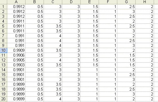
sorted by the first column, the correlation coefficient. The sorted file is
shown in Fig. 3. The values in columns B through H are the system
parameter values, corresponding to the first seven inputs of the
IdealEqtyOpt5 function, as shown above. The values in the top row, which has the
highest value of the correlation coefficient, are the optimal
results.

Figure 3. Spreadsheet
file of results from the IdealEqtyOpt5 function. The file is sorted by column A,
the correlation coefficient. The remaining columns contain the system parameter
values.
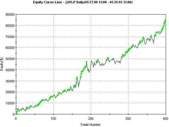
The equity curve
based on the optimal set of parameter values is shown below in Fig. 4. As
intended, using the IdealEqtyOpt5 function resulted in a
very linear equity curve.

Figure 4. Optimal
one-contract equity curve for the MiniMax system on daily bars of US
T-Bonds (symbol @US.P in TradeStation 8) for trades on the optimization segment
(15 years ending 5/26/1995). $75 was deducted from each trade for slippage and
commissions.
The corresponding performance
over the optimization period is as follows:
Net Profit:
$86,806
Profit Factor:
1.6
Percent Wins: 54.5% (398 trades
total)
Ave. Trade:
$213
Win/Loss: 1.35
Max Intraday Drawdown:
$11,275
To determine how well the
optimal results are likely to hold up going forward, the system was run over the
last 10 years of T-Bond data, from 5/28/1995 to 5/31/05. These "out-of-sample"
data were not used in the optimization, so they provide a more objective measure
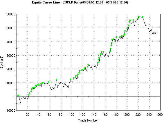
of the system's performance than the results over the optimization segment. As
shown in Fig. 5, the equity curve in the out-of-sample period is also quite
linear until it enters a drawdown period in recent trading.

Figure 5. Out-of-sample
one-contract equity curve for the MiniMax system on daily bars of US
T-Bonds (symbol @US.P in TradeStation 8) for trades on the 10-year data segment
ending 5/31/2005 using the optimal parameter values. $75 was deducted from
each trade for slippage and commissions.
The corresponding performance
over the out-of-sample period is as follows:
Net Profit:
$47,569
Profit Factor:
1.4
Percent Wins: 53.2% (252 trades
total)
Ave. Trade:
$189
Win/Loss: 1.23
Max Intraday Drawdown:
$15,269
Compared to the EqtyCorr
function I presented last November, IdealEqtyOpt5 does not require the
selection of any weighting factors and is therefore simpler. It also has the
advantage of relating the optimal results to the profit potential of the market.
By the way, in the optimization segment, there were 398 system trades and
408 ideal trades. If the number of system trades had been much different than
the number of ideal trades, the ATR fraction (function input
RevFr) could have been adjusted to bring the numbers closer together.
On the other hand, the EqtyCorr function was more versatile in that the
weighting factors could be used to bias the optimization to the most recent time
period. A similar effect could be achieved in IdealEqtyOpt5 if desired by
weighting the ideal equity curve.
As with any trading
system optimization, it's always a good idea to save some data
for out-of-sample testing and preferably track the system in real-time before
committing real money.