The Breakout
Bulletin
The following article was originally published in the December 2005 issue of
The Breakout Bulletin.
Create
Your Own Price Data: Creating and Using Synthetic Price Data
One of the problems often
encountered when developing and testing trading systems is insufficient data to
produce reliable test results. As I've discussed before in this newsletter,
system testing results are more reliable with more data. Generally speaking, the
more data we can test on, the better. In his book "Beyond Technical Analysis,
2nd Ed.," Tushar Chande addresses this problem by demonstrating how to develop
synthetic price data using a method he calls "data scrambling" [reference 1].
His basic idea is to start
with an actual price series and randomly sample from it to create a "synthetic"
price series. However, rather than sampling the prices directly, we sample from
the price changes. Consider the spreadsheet shown below in Fig. 1.
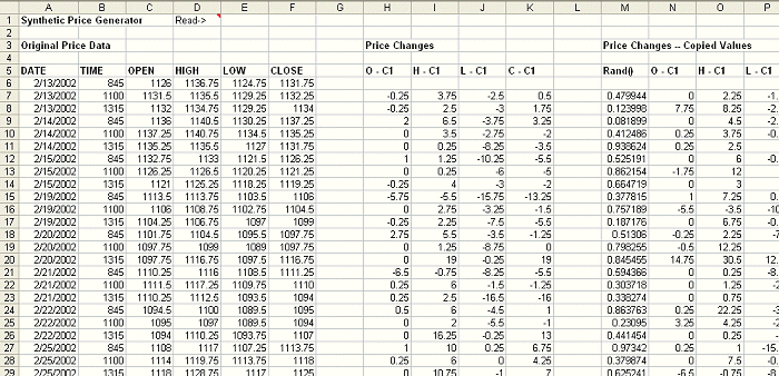
Figure 1. Spreadsheet for creating synthetic price data. Original price data (A
- F) is converted to price changes (H - K).
The first six columns
contain the original price data. Columns H - K convert the price data into price
changes by subtracting the close of the previous bar. For example, the open
becomes the open minus the previous close. The high becomes the high minus the
previous close, and so on. It's necessary to work with price changes rather than
absolute prices in order to preserve the price changes from bar to bar.
After calculating all the
price changes, the next step is to randomize the order of the price changes.
This is a little different from the method proposed by Chande who describes
using random sampling with replacement. In sampling with replacement, you would
randomly select rows from the price change columns and use those to construct
the new prices. In sampling with replacement, you might select the same row more
than once. Randomizing the order of the price changes is random sampling
without replacement. This means we randomly sample from the price changes,
but we select each row exactly once.
To do this in the
spreadsheet, we copy the columns containing the price changes (H - K) and paste
the values into new columns (N - Q); see Fig. 2 below. The important point is
that we paste the values only -- not the formulas. We then add an additional
column (M) to the left of the copied columns to contain random numbers.
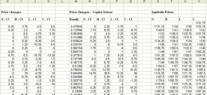
Figure 2. Continuation of spreadsheet from Fig. 1. Price changes (H - K) are
copied (values only) to columns N - Q and used to create synthetic prices (S -
V).
Random numbers can be
produced in Excel using the Rand() function. Now that we have the price changes
and the column of random numbers, we select the four columns of price changes
plus the column of random numbers (M - Q) and sort the columns (Sort command,
Data menu) by the column of random numbers (M). This will randomize the order of
the price changes. Notice that we sort the columns of price changes together, so
the data for each bar stay together.
Finally, the synthetic
prices are generated by adding the price changes back to the closing prices. For
example, the Open - Close price change is added to the prior close to create the
synthetic open price. We start with a reference closing price, which is used for
the first row. In Fig. 2, the reference closing price is 1131.75, which appears
by itself at the top of the "Synthetic Prices" section in column V. Subsequent
rows are created by adding the price changes in that row to the closing price
for the prior row. In this way, each price bar is relative to the previous bar's
close.
As an example of the type of
price data this produces, consider Figs. 3 - 6. Fig. 3 is price plot of the
original data. Figs. 4 - 6 contain three different sets of synthetic prices
generated by randomizing the price changes of the original data as described
above.
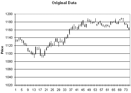
Figure 3. Original price data.
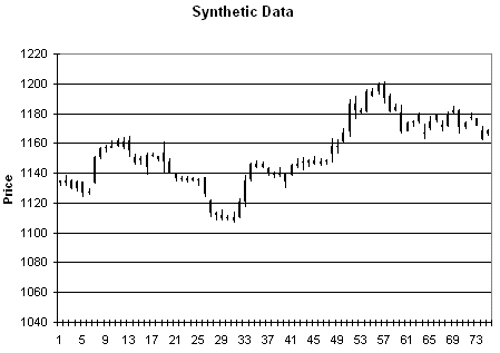
Figure 4. Synthetic
prices generated from the data in Fig. 3.
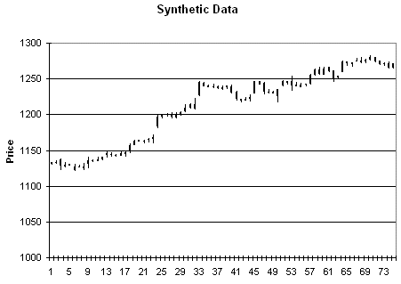
Figure 5. Synthetic prices generated from the data in Fig. 3.
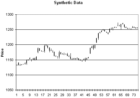
Figure 6.
Synthetic prices generated from the data in Fig. 3.
The spreadsheet that
performs these calculations is located on the
Free Downloads page on my web site. To use the spreadsheet,
follow the instructions in the comment near the top of the spreadsheet in cell
D1, which contains "Read ->". Basically, all you need to do is copy your own
price data over the data in the spreadsheet, then copy the price change columns
to the columns labeled "Price Changes -- Copied Values." Make sure to copy the
values only. Fill down as needed or delete rows if your data require more or
fewer rows than the data already in the spreadsheet. Then select the copied
price change columns and the column of random numbers (M - Q) and sort
everything by the column of random numbers (M). To recreate a valid file or
price data, copy the synthetic prices (S - V) back into your original file of
data next the date/time columns. This will produce a file of synthetic prices
with valid dates/times.
A few points about this
approach are worth discussing. First, this method preserves not only the price
changes but the price relationships within each bar. It's basically randomizing
the order of the bars but keeping each bar the same. The only price
characteristic that's being altered is the ordering of the bars. The advantage
of this approach is that it preserves quite a lot of information about the price
series while generating different price formations in the new, synthetic series.
However, if you have a trading system that's based on price patterns or methods
that depend on a specific ordering of the price bars, there's no reason to think
your system will hold up when tested on the synthetic data. For example, if
you've found that four up closes in a row is a valid buy signal, you probably
shouldn't expect to find that result in a synthetic price series. If that
particular price pattern is useful, it's probably because it captures some
nonrandom market tendency, such as a psychological response to a strong,
short-term trend. If you randomize the price changes, you'll lose that pattern
in the synthetic price series.
Also, while the synthetic
price series may look much different than the original price series, it still
contains the same statistical distribution of price changes. Over time, markets
change. One characteristic that can change is the distribution of price
changes. Synthetic data as described here won't address that.
Applications of
Synthetic Price Data
Keeping in mind the points
just made, there are two applications of synthetic price data that I'll
discuss. The first application is the one recommended by Chande [reference 1];
namely, using synthetic data for system testing. Chande describes this use as
true out-of-sample testing. Certainly, a system that performs well on synthetic
price data is more robust than one that only does well on historical data. It
implies that the system is insensitive to the kind of price-change randomization
used to generate the synthetic data. Generally speaking, the more market
characteristics that a system is insensitive to, the better. For example, if I
had a system that was insensitive to price volatility, it would be better than a
system with similar performance that could break down with changes in
volatility. A system that holds up well when the price changes are re-ordered,
as with a synthetic price series, is better than a system that breaks down on
synthetic data. However, there's no guarantee that a system that performs well
on synthetic data will hold up as well in the future. As noted above, the
distribution of price changes could drift over time or even change suddenly, and
synthetic prices can't test for this.
Provided you're testing a
system that should in principle hold up on synthetic data, I would suggest an
extension of Chande's approach. Instead of just testing a system on synthetic
data, why not create a very long synthetic price series and optimize the
system's parameter values on the synthetic price series? How long a series is
necessary? As noted in previous newsletters, the more trades used in the
optimization, the better. If you can create a synthetic price series that
generates 500 trades, that would be better for optimization than one with only
100 trades. After optimization, test the system with the optimized parameter
values "out-of-sample" on the actual price data. To provide even better
out-of-sample testing, divide the original historical data into two segments.
Use the first segment to create the long, synthetic price series for
optimization. Save the second segment for true out-of-sample testing of the
optimized system. This has the following advantages:
-
You're optimizing
over a long price history that generates a large number of trades.
-
The price data
include random patterns so the resulting parameter values will not be
fit to a small number of historical price patterns that may never
repeat.
-
By saving the actual
historical data for out-of-sample testing, your final test results will
give you confidence that the system is capable of performing well on
"real" data.
In principle, one of the
advantages of synthetic prices is that you can create arbitrarily long series.
To do this in practice using the spreadsheet described above can be a bit
tricky, however. Here's one way to do it. Copy the data in the price change
columns (N - Q) and paste the data directly below the existing numbers in the
same columns, which will double the length of the columns. Repeat the process as
many times as necessary to get the length you want. Then fill-down the random
number column (M) and the synthetic price columns (S - V). Now sort the price
change columns (N - Q) by the random number column (M). This will randomize the
price changes and produce the synthetic prices in columns S - V. The only
problem is that you'll need to assign dates/times to the prices in order to
create your finished price file. If the data are daily bars, so that each bar
has a different, consecutive date, this is relatively easy. Convert the dates to
numbers by formatting the date column as "text." Then increment each date value,
which is now a number, by 1, starting at the last row for which you have date
information available. For example, if the last row for which you have dates is
row 546 and the date is 11/21/2005, then you would convert this date to a number
(in this case, it's 38677) by formatting the cell as text. Then you set the
date cell for the next row to A546 + 1 (assuming dates are in column A). The
date for the next row would be A547 + 1, etc. You can fill down this formula to
increment the date by 1 in each successive row. Then reformat the cells as
"dates." Intraday data may require a little more work because several rows of
data will have the same date, but the idea is the same.
The second application for
synthetic price data that I want to discuss is testing price patterns. Above, I
suggested that if your trading system is based on a price pattern that relies on
a specific pattern of relative prices, then you'll probably lose that pattern
when you randomize the price changes to create the synthetic price data. In this
case, our goal is not to come up with a system that is insensitive to price
change patterns, as it would be if we were using synthetic data to optimize our
system. Quite the opposite. We've found a price pattern that we believe
represents some sort of nonrandom market phenomenon, and our goal is to
determine if the pattern has any validity.
Let's say, for example, that
we've found a pattern that seems to predict that the market will be higher five
days later with 60% accuracy. We need to know if 60% accuracy is meaningful or
if we could get that kind of accuracy just by random chance. If random chance
can produce that kind of accuracy, then our price pattern is not meaningful.
This is where the synthetic price data come in. Because the synthetic price data
are generated by randomizing the price changes, we can search for our pattern on
the synthetic data to determine the accuracy of the pattern on random prices. In
order for our price pattern to be meaningful and not just a byproduct of random
chance, the pattern should have a higher accuracy on the real data than on most
(in a statistical sense) of the synthetic price data.
As an example, we'll
consider a pattern for the E-mini S&P 500 futures on 135 min bars over the date
range 2/13/2002 to 11/21/2005. 135 min bars divide the day session evenly into
three parts (think morning, mid-day, and afternoon session).
The price pattern
is as follows:
Lowest low of the
last 20 bars is found within the past 5 bars
High - low range
less than the average high - low range over the past three bars
Close above previous
close
Close above average
close over past 180 bars
We'll evaluate this pattern
by calculating the probability that the market is higher five days later.
Results
On Original Data:
65.4% of time (34 of 52
patterns), close was higher 5 days later.
On Synthetic Data:
Series
Probability of higher close 5 days later
1 55.9%
2 50.0
3 50.0
4 40.8
5 49.1
6 49.1
7 50.0
8 50.0
9 42.9
10 40.8
Each series consisted of a
different synthetic price series created from the original data. Over all 10
series, the average probability is 47.86 +/- 4.83%. In other words, averaging
those 10 probability results, the average accuracy of the 10 series is 47.86%
and the standard deviation is 4.83%. Ideally, we'd like to have about 30 series
to ensure that the distribution is statistically valid, but for the sake of
illustration, we'll assume these 10 are sufficient.
In general, 99.9% of
normally distributed data are less than three standard deviations above the
mean. In this case, three standard deviations above the mean is 47.86 + 3 * 4.83
or 62.4%. In other words, 99.9% of the results from the synthetic price series
will be less than 62.4%. Since our accuracy on the actual data was 65.4%, the
accuracy of our price pattern is greater than 99.9% of the accuracy values
calculated from the synthetic data, which implies that the accuracy is not due
to random chance but due to some other phenomenon. This should give us some
reassurance that the price pattern is capturing something other than just random
noise.
The two uses of synthetic
price data described here for evaluating trading systems are quite different
from one another. In one case, we're testing or optimizing our trading system on
the synthetic prices with the expectation that our system will perform well even
on the randomly generated synthetic data. In the other case, we expect that our
price pattern will only work well on the original data. Clearly, the way we use
synthetic data of the type described here depends on the kind of system we're
analyzing. Provided you keep this fact in mind, synthetic price data can be a
useful tool to help develop and analyze your trading systems.
Reference
1. Tushar Chande, Beyond
Technical Analysis, 2nd ed., John Wiley & Sons, Inc., New York, 2001, pp.
346-352.
That's all for
now. Good luck
with your trading.
Mike Bryant
Breakout Futures
 |