Trading Rules from Statistical Grouping
of Indicators
A
while back I started thinking about the mathematical characteristics of neural
networks. One of their key characteristics is that they use a complex, nonlinear
function to capture patterns in the market that are not obvious with more
conventional methods. The nonlinear function combines a set of inputs, typically
based on indicators (e.g., moving averages, stochastics, momentum, and so on),
into a single output that ranges from -1 to +1. To use this output in trading,
we can look for long entries when the function output is above +0.5 and for
short entries when the function output is below -0.5.
Transforming the multiple inputs into a single output is a continuous, nonlinear
function. Trying to fit this single continuous function to different sets of
market conditions simultaneously so that the network properly assigns bullish
conditions to output values greater than 0.5 and bearish conditions to output
values less than -0.5 is quite challenging, to say the least. In my experience
there are many different sets of conditions that set up profitable long trades
and many other sets of conditions that set up profitable short trades. Perhaps
it's asking too much of a single continuous function to somehow weave a twisted
path among disparate sets of market conditions.
This
led me to wonder if the neural network approach could be adapted to
"discrete"-value functions. In other words, rather than using a continuous
function, the function would have a small number of values, perhaps each one
corresponding to a different set of market conditions. One way to approach this
is by grouping the data into "bins," similar to the method I used in the article
on Dynamic Portfolio
Selection.
As an example, suppose
we have the following set of five indicators:
I1 = C - C[1]
I2 = C - C[3]
I3 = C - AMA
I4 = AMA - Average(C, 30)
I5 = TrueRange -
Average(TrueRange, 30)
where C is the closing
price of the current bar, C[1] is the close one bar ago, C[3] is the close three
bars ago, AMA is an adaptive moving average based on a variable speed
exponential moving average, as calculated by the TradeStation built-in function
AdaptiveMovAvg(C, 20, 2, 40), Average(C, 30) is the simple moving average of the
last 30 closing prices, TrueRange is the true range of the current bar, and
Average(TrueRange, 30) is the simple moving average of the true range over the
last 30 bars.
If we determine the
minimum and maximum values for these indicators over our data set, we can scale
the indicators so that they lie in the range -1 to +1, denoted [-1, +1]. For
example, to scale I1 into this range, we can write:
I1scale =
(2 * I1 - (SfMax1 + SfMin1))/(SfMax1 - SfMin1)
where SfMax1 and SfMin1
are the maximum and minimum values, respectively, of I1.
Now that the indicators
all produce values in the range [-1, +1], we can group them into bins based on
their values. Suppose we divide the range into the following four bins: [-1,
-0.5], (-0.5, 0], (0, +0.5], (+0.5, 1]. So, if an indicator is greater than or
equal to -1 and less than or equal to -0.5, it lies in bin #1, [-1, -0.5]. If
the indicator is greater than -0.5 and less than or equal to zero, it lies in
bin #2, (-0.5, 0]. Values greater than zero and less than or equal to 0.5 lie in
bin #3, (0, +0.5]. Finally, if an indicator is greater than 0.5 and less than or
equal to 1, it lies in bin #4, (+0.5, 1].
The basic idea of this
approach is to evaluate the five indicators on the bar prior to each trade we
want to take. To keep things simple for illustrative purposes, I'll assume the
trades enter on the day's open and exit at the close on the same day. Provided
we're using intraday data, this means we want to evaluate the indicators on the
last bar of each day in preparation for entering on the next day's open.
When we evaluate the
indicators, we'll determine into which bin each one falls. We'll keep track of
the bins for each indicator for each trade. We'll also keep track of the
profit/loss amount for each trade. At the end, we'll find the combination of
bins that produced the greatest net profit. For example, it might turn out that
when the five indicators were in bins 3, 1, 2, 1, and 4, respectively, we
obtained the most profit buying on the open (i.e., going long). By taking the
negative value of the profit/loss amounts, we can use the same data to find the
best bin combination for going short on the open.
Notice that the number
of possible bin combinations is the number of bins raised to the power of the
number of indicators, or 4^5 = 1024 combinations in our example. It will turn
out that only a relatively small number of these combinations contain more than
one trade. We want to focus on the combinations that contain a reasonably large
number of trades so the results will be more significant.
I wrote a strategy in
TradeStation called StatBins1 to perform the calculations. This strategy can be
downloaded from my web site on the
free downloads page. Instructions for applying
the strategy are provided in the lengthy comment at the top of the strategy
code.
After finding the
scaling factors, I ran StatBins1 on 60 minute bars of the e-mini Russell 2000
futures over the past five years, ending 12/15/2006, with a lookback length of
50. The strategy produced the following results, which were written to the
TradeStation Print Log:
StatBins1...
Total Number of Simulated Trades = 1239
Combo Total Long P/L No. Trades
22 4550.00 7
23 -1390.00 3
27 -510.00 4
66 -1100.00 2
70 1170.00 32
71 -2570.00 5
82 530.00 2
86 2810.00 97
87 -5860.00 41
90 -14130.00 46
91 480.00 82
102 -5160.00 28
103 1520.00 14
106 -8890.00 60
107 -2650.00 133
111 -3830.00 10
123 -840.00 8
127 -580.00 3
134 -690.00 21
135 3800.00 6
139 2170.00 2
146 -2100.00 2
150 6420.00 76
151 6210.00 34
154 2280.00 38
155 8000.00 46
166 3220.00 26
167 3000.00 15
170 -4710.00 81
171 -10100.00 158
186 300.00 2
187 990.00 14
234 1810.00 10
235 1330.00 14
326 -630.00 10
342 -1920.00 14
343 660.00 3
346 160.00 3
347 680.00 6
363 1320.00 10
367 -830.00 2
386 220.00 3
390 1370.00 5
406 -1060.00 9
410 1140.00 2
411 1470.00 7
422 1090.00 2
426 2120.00 3
427 -920.00 14
491 1520.00 3
Bins (0 - 3): [-1, -.5] (-.5, 0] (0, .5] (.5, 1]
Maximum Profit/Loss, Long: 8000.00
Bins: 2 2 1 2 0
Number of trades: 46
Maximum Profit/Loss, Short: 14130.00
Bins: 1 2 1 1 0
Number of trades: 46
The
first part of the output is a table of bin combinations, with the combinations
numbered from 1 to 1024.The table lists the net profit and number of trades for
bin combinations with more than one trade. Combinations with positive net profit
amounts represent net profitable long trades, whereas negative amounts represent
net profitable short trades. Following the table, the combination with the
greatest net profit is shown for both long and short trades. For example, the
best bin combination for long trades was when indicator I1 was in bin 2,
indicator I2 was in bin 2, indicator I3 was in bin 1, indicator I4 was in bin 2,
and indicator I5 was in bin 0 (the bins are numbered from 0 to 3 in the
strategy).
To
see more detailed performance results for the optimal bin combinations,
theStatBins1 strategy can optionally be run as a system by entering the optimal
bin numbers as inputs to the strategy and setting the input "TradeIt" to TRUE.
When this is done, StatBins1 uses the indicators and bin numbers to take trades
when the indicators lie in the specified bins. Trades are entered at the open
and exited at the close. No stop is used.
With
$25 per round turn deducted for slippage and commissions, StatBins1 produced the
following results on a one-contract basis using the optimal bin combinations
shown above:
Net Profit: $19,830
Profit Factor: 2.28
Number of Trades: 92
Percent Profitable: 63.0%
Average Trade: $215
Ave Win/Ave Loss: 1.34
Worst-case Intraday
Drawdown: -$3,040
The
equity curve is shown below in Fig. 1.
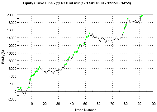
Figure 1.
StatBins1 optimal trading results on ER2, 60 min, five years ending 12/15/06,
with $25 trading costs.
Although in the example
presented here, the indicator bins were used as the sole trade entry
criterion, it's probably better to combine this approach with other entry and
exit techniques. For example, the StatBins1 code could be modified to track the
bins prior to entering trades on a breakout or using other criteria. In that
way, the indicator bin values would serve as a filter for the primary entry
technique. More sophisticated exit techniques could be added as well.
Also note that the
results shown above are in-sample, optimized results. Using the bin values that
generate the greatest net profit is optimization. Out-of-sample testing and
real-time tracking are always a good idea before committing real money to any
new trading approach.