Was January Unusual?

I spoke with several traders in February who remarked that the market seemed to be trading differently (and not "good" different). The consensus seemed to be that the worries about war with Iraq were affecting the markets and making them more difficult to trade. This made me wonder if there was a way to quantify the apparent changes in market behavior. Towards this end, I looked at several indicators that represent market dynamics.

False Breakout Indicator

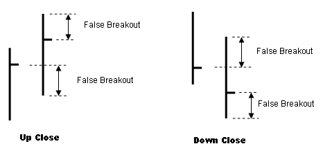
To get a better feel for the extent of false breakouts recently, I came up with an indicator that quantifies the size of the false breakouts, if any, on each bar. I define a false breakout as the amount the market moves in the direction opposite to the direction in which the bar eventually closes or the amount the market moves beyond where it eventually closes. Specifically, on an up bar, I define a false breakout as the amount that the market drops below the prior close or rises above the current close, whichever is larger. Similarly, on a down bar, the false breakout is the amount the market rises above the prior close or drops below the current close, whichever is larger. This is illustrated in Fig. 1. A bar that closes at the high or low of the day and has no trading overlapping the prior close would have a zero value of the false breakout. To create the indicator, I plot the raw value on each bar normalized by the average true range and the moving average of this value. ("Range" is simply the bar's high minus it's low; "true range" is similar but takes gaps into account.)

Fig. 1 Defining "false breakouts" for the FalseBreakout indicator.

The EasyLanguage code for the FalseBreakout indicator is shown below.

{
  Indicator: FalseBreakout
  This indicator calculates the size of the false breakout
  on each bar (if any). It normalizes the result by the
  average true range and plots the raw value plus the
  average.
 
  Michael R. Bryant
  Breakout Futures
  www.BreakoutFutures.com
  Copyright 2003 Breakout Futures

  Feb 11, 2003
}

  Input: N    (10);
 
  Var: FBO     (0),
       AFBO    (0); 

  If C >= C[1] then
     FBO = MaxList(H - C, C[1] - L)
  else
     FBO = MaxList(H - C[1], C - L);

  FBO = FBO/Average(TrueRange, N);
  AFBO = Average(FBO, N);

  Plot1(FBO, "False B/O");
  Plot2(AFBO, "Ave B/O");

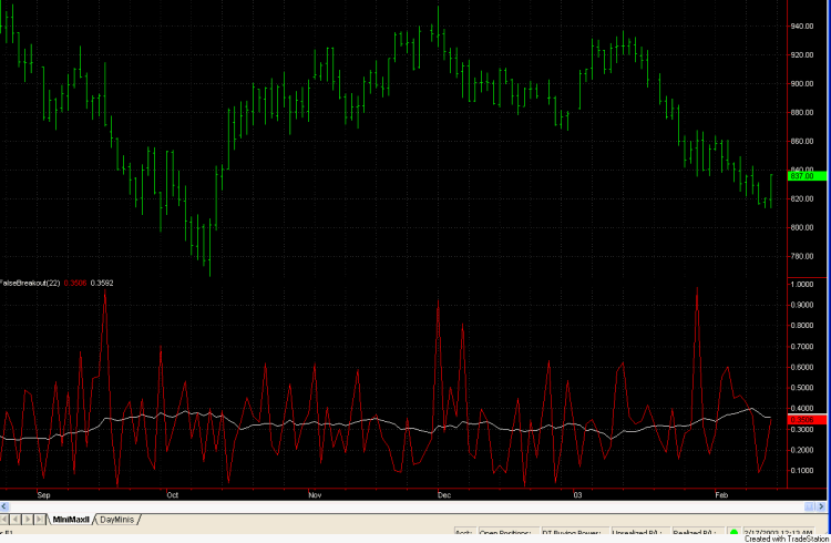
Fig. 2 shows what this looks like on daily bars for the E-mini S&P over recent months. While the daily value is quite volatile, the average value doesn't change much over time, suggesting that there have been no more false breakouts recently than in the past. While my subjective impression was that there were more false breakouts in January than usual, this is not supported by the false breakout indicator.

Fig. 2. FalseBreakout indicator plotted on a chart of daily bars of the E-mini S&P.

Trendiness Indicator

A common way to define the strength of the market trend is to divide the absolute value of the change in price by the average true range over the past N bars. This tells us how much the market has moved relative to the average true range. A market that's moved three times the average true range over the last month has a stronger trend, for example, than one that's moved only 1.5 times the average true range.

In EasyLanguage, this can be written as follows:

  Input: NBars (30);
 
  Value1 = AbsValue(C - C[NBars])/Average(TrueRange, NBars);

  Plot1(Value1, "Trendiness");

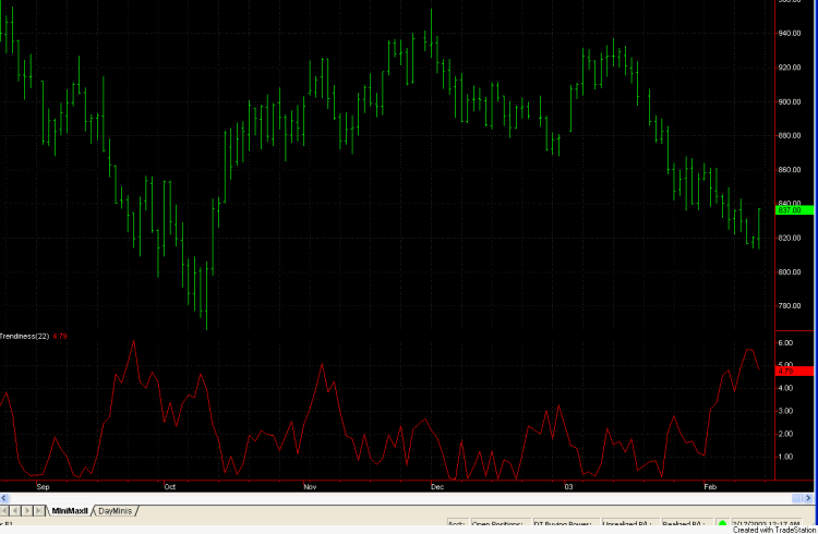
In Fig. 3, this indicator ("Trendiness") is plotted on a chart of daily E-mini S&P data using a look-back period of 22 days, the average number of trading days in a month. The indicator looks particularly flat during December and January, two difficult months for the short-term trading approach of the MiniMax II system. In fact, the indicator only briefly got above a value of 3 over this 2-month period. The last time the indicator was consistently this low was over the Dec-Jan period one year earlier. Interestingly, MiniMax II was modestly profitable during that period. The lack of trend strength may be a distinguishing factor in the recent Dec-Jan trading period. However, it's not entirely clear that lack of trend strength correlates strongly with lack of good trading opportunities.

Fig. 3. Trendiness indicator plotted on a chart of daily E-mini S&P data.

Average True Range Indicator

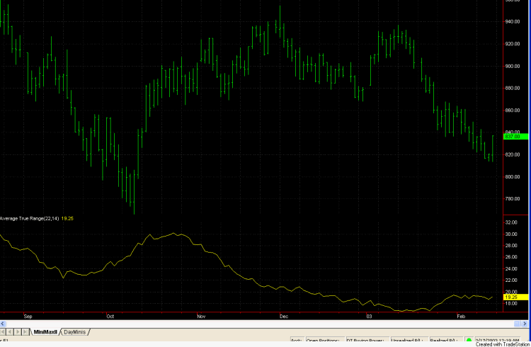
The last indicator I want to examine is the average true range. In Fig. 4, the average true range (ATR) is plotted for the daily E-mini S&P using a look-back period of 22 days. In my opinion, this is the most striking of the three indicators. The ATR hit a low of 16.7 (E-mini S&P points) on Jan 14th and is currently hovering around 19. This is the lowest value since Mid-April 2002 and is nearly half the value we saw in mid-October and early August. The ATR has been trending steadily downward since mid-October, only recently appearing to bottom out in January. While the trading volume of the E-mini S&P is about as high as ever, the daily ranges have been contracting. One possible interpretation of this is that it represents a lack of conviction among investors and traders. Whatever the reason, it raises several questions. Is the lack of volatility temporary? If it persists, how will it affect trading? Is there a way to compensate for it? I try to address the last question below.

Fig. 4. Average true range plotted on a chart of daily E-mini S&P data.

Dealing With Declining Volatility

In this section, I present two methods to adapt a trading system to market volatility. These methods -- the second one in particular -- are best suited to breakout systems, although they may be worth investigating for other types of systems as well.

Cycles of Volatility

In the November issue of this newsletter, I discussed using the ATR as a filter for a simple breakout system. The idea is based on the observation that the ATR is mean reverting; that is, it tends to move back to its average value if it gets too far away from it. If the ATR is low, it will most likely move higher over the next few bars, and vice-versa if the ATR is high. This suggests that if you wait until the ATR is low, a breakout trade entering on the next bar has a better chance of developing into a nice trade. I demonstrated that at least for the simple system I presented, using the ATR in this manner helped improve the overall performance.

An even better way to take advantage of cycles of volatility is to use the product of volume and ATR. I refer to this product as the "activity." For example, a day with a large range and lots of volume is arguably more "active" than a day with the same range but low volume. Similarly, a day with high volume but a low range is less active than a day with the same volume but a large range. To provide a "trigger" level, I take the average of the activity over the last N days. Because the activity is mean-reverting, if the activity is below its average, the activity can be expected to increase over the next few bars. This can be used as an entry filter to help restrict your trading to more active days. Specifically, look for a breakout on the next bar if the activity on the current bar is below its N-bar moving average.

In EasyLanguage, this filter can be written as follows:

Var: NAct       (30),    { look-back period for activity indicator }

     ActInd     (0);     { value of activity indicator }

ActInd = TrueRange * Volume - Average(TrueRange * Volume, NAct);

If ActInd < 0 then

  { Place the entry order here; e.g., Buy next bar at H stop; }

I've tried this filter on several different breakout-type system, and it improved the performance in each case. It might be worth trying with your own system.

Adapting the Breakout Amount to Volatility

A classic entry method is to enter on a breakout from yesterday's high, low, or close by an amount given by a multiple of the prior day's range or average range. For example, you might take 50% of yesterday's range, and add it to yesterday's high to define your long entry price. Since the amount of the breakout is a multiple of the range, this method inherently adapts to the market's volatility, as defined by range or true range. However, there's no rule that says this type of simple, linear function of volatility is an adequate way to adapt the size of the breakout to the volatility. For example, if low volatility is an indication of lack of conviction by traders, we might expect that we'll get more poor quality trades in a low-volatility market as the expected trends fail to materialize. This is probably what happened to the MiniMax II system in January. Under these conditions, we might want to increase the size of our breakout when the market declines in volatility in order to raise the threshold for entry and avoid trades in a trendless or reversal-prone market. However, this is exactly the opposite of what will happen when we take our breakout based on a simple fraction of the true range or ATR. Basing the breakout on a simple fraction of the true range or ATR results in smaller breakouts as the volatility declines.

Here's one possible solution. Instead of taking a breakout as a simple fraction of volatility, make the fraction a linear function of volatility, with a larger fraction at low volatility and a smaller fraction at high volatility. The breakout itself is still calculated the same way, by multiplying the ATR or true range by the fraction. However, the fraction will vary with the ATR.

As a baseline for comparison, consider the simple breakout system below:

Input:  EntFrL    (1.0),  { Volatility multiplier for entry }
        EntFrS    (1.0),  { Volatility multiplier for entry }
        MMFrL     (2.0),  { Volatility multiplier for exit }
        MMFrS     (2.0);  { Volatility multiplier for exit }

Var:    ATR       (0);    { average true range }

ATR = Average(TrueRange, 22);

Buy next bar at H + EntFrL * ATR stop;
Sell short next bar at L - EntFrS * ATR stop;

If MarketPosition = 1 and C > EntryPrice and BarsSinceEntry >= 1 then
   Sell this bar at close;

If MarketPosition = -1 and C < EntryPrice and BarsSinceEntry >= 1 then
   Buy to cover this bar at close;

If MarketPosition = 1 then
   Sell next bar at EntryPrice - MMFrL * ATR stop;
 
If MarketPosition = -1 then
   Buy to Cover next bar at EntryPrice + MMFrS * ATR stop;

This system enters on a breakout from the prior high/low using a fraction of the 22-bar ATR as the amount of the breakout. It exits on the first profitable close after at least one bar if not stopped out at the exit stop given by a fraction of the ATR from the entry. Using 1410 min bars of the E-mini S&P (symbol @ES in TS 6; a 1410 min bar represents one day), I optimized the inputs over the last 500 days. I found the following input parameter values worked well: EntrFrL = 0.4, EntrFrS = 0.3, MMFrL = 0.6, and MMFrS = 1.9. The one-contract results using these inputs were as follows ($75 per contract has been deducted for trading costs):

Net Profit: $16,863

No. Trades: 155

% Winners: 68%

Ave. Trade: $109

Profit factor: 1.39

Max Drawdown: -$6,038

We'll take these as the baseline results without the variable breakout fraction. Now consider the system with the variable breakout fraction.

 Input: FrLv0     (.8),   { Breakout fraction, low vol, longs }
        FrLv1     (.3),   { Breakout fraction, high vol, longs }
        FrSv0     (.8),   { Breakout fraction, low vol, shorts }
        FrSv1     (.3),   { Breakout fraction, high vol, shorts }
        MMFrL     (2.0),  { Volatility multiplier for exit, longs }
        MMFrS     (2.0);  { Volatility multiplier for exit, shorts }

 Var:   ATR       (0),    { average true range }
        ML        (0),    { slope of b/o fraction curve, longs }
        BL        (0),    { y-intercept, longs }
        MS        (0),    { slope of b/o fraction curve, shorts }
        BS        (0),    { y-intercept, longs }
        V0        (16),   { low volatility }
        V1        (30),   { high volatility }
        FrL       (0),    { entry fraction for longs }
        FrS       (0);    { entry fraction for shorts }

 ATR = Average(TrueRange, 22);
 ML = (FrLv1 - FrLv0)/(V1 - V0);
 BL = FrLv0 - ML * V0;
 MS = (FrSv1 - FrSv0)/(V1 - V0);
 BS = FrSv0 - MS * V0;
 FrL = ML * ATR + BL;
 FrS = MS * ATR + BS;

 Buy next bar at H + FrL * ATR stop;
 Sell short next bar at L - FrS * ATR stop;

 If MarketPosition = 1 and C > EntryPrice and BarsSinceEntry >= 1 then
    Sell this bar at close;

 If MarketPosition = -1 and C < EntryPrice and BarsSinceEntry >= 1 then
    Buy to cover this bar at close;

 If MarketPosition = 1 then
    Sell next bar at EntryPrice - MMFrL * ATR stop;
 If MarketPosition = -1 then
    Buy to Cover next bar at EntryPrice + MMFrS * ATR stop;

This system uses a simple linear equation to calculate the breakout fraction as a function of ATR. ML (MS) and BL (BS) are the slope and "y-intercept" of the linear equation for long (short) trades. Instead of a single value of the breakout fraction as a system input, this system uses two values: FrLv0 (FrSv0) and FrLv1 (FrSv1) for long (short) trades. The first parameter is the value of the breakout fraction at low volatility, and the second parameter is the value of the fraction at high volatility. I've somewhat arbitrarily defined "low" and "high" volatility as ATR values of 16 and 30, respectively (variables V0 and V1). The exit logic is identical to the baseline system above.

I left the exit parameter values the same as in the baseline system: MMFrL = 0.6 and MMFrS = 1.9. I couldn't find any better parameters for the short side than the 0.3 value that worked well in the baseline system, so I used FrSv0 = FrSv1 = 0.3. However, for the long side, I found that the parameters FrLv0 = 0.5 and FrLv1 = 0.4 worked well. Compared to the baseline system, the only difference is that the breakout fraction for long trades varies between 0.5 when the volatility is low to 0.4 when the volatility is high.

With this one change, the one-contract results over the same period of time as for the baseline system are as follows ($75 per contract has been deducted for trading costs):

Increasing the breakout fraction under conditions of low volatility improves the performance of this system on the long side of the market. The improvement appears to results from filtering out 14 trades that the baseline system took. This is consistent with our goal of avoiding poor trades during periods of low volatility. This idea may be worth testing on other systems and markets. One drawback is that you introduce extra input parameters. However, as long as any parameter optimization is performed over a large number of trades, as in the examples here, the risk of over-fitting the system to the market is minimal. As with any trading approach, it's probably a good idea to test it in real time before committing capital.

In summary, the markets have exhibited declining volatility in recent months. While this lower volatility may cause problems for some short-term trading systems, there may be ways to mitigate the damage. Hopefully, you'll find one or both of the ideas I've discussed here worth investigating for your own trading. That's all for now.