Breakout Bulletin - March 2005

A Rapid Prototyping Method for Trading System Development

The usual approach to developing a trading system is to start with an idea about how the markets works. You then try to translate that idea into a set of trading rules, add one or more exit strategies, perform some testing, and make adjustments as necessary. If you're lucky, the initial idea was sound, and the system will work. In my experience, however, most ideas simply don't hold up. I've discarded more trading system ideas than I care to remember. Wouldn't it be nice if there was a way to rapidly test multiple trading ideas in one system, rather than coding and testing a separate system for each idea?

In this article, I'll present a method for doing just that. I call it a rapid prototyping method for trading system development. As you'll see, it can be used to find a viable set of trading rules for a system starting with a basic set of indicators. You can also use this method to search for profitable price patterns. The method takes advantage of the built-in optimization feature of TradeStation to iterate through all possible combinations of a set of indicators or price relationships to find the combinations that work best.

To begin, I assume that the entry rules for a trading system can be represented by a set of conditions. If all the conditions are true, the trade is entered. I also assume that for systems that have both long and short trades the entry conditions for the short side are the logical opposite of those for the long side. More specifically, I'm interested in entry conditions that can be represented by inequalities. For example, C < C[2] ("Close is less than close of two bars ago") or Average(C, 5) < Average(C, 25) ("Average close over the last 5 bars is less than the average close over the last 25 bars"). Not all entry conditions fit this mold, but many do.

Under these assumptions, the buy and sell entry signals for a trading system can be represented by the following logical (true/false) variables:

BuySig = w1 * C1 >= 0 and w2 * C2 >= 0 and ... wn * Cn >= 0

and

SellSig = w1 * C1 <= 0 and w2 * C2 <= 0 and ... wn * Cn <= 0

where BuySig is the signal for entering a long trade, and SellSig is the signal for entering a short trade. In other words, if BuySig is true, a long trade is entered. If SellSig is true, a short trade is entered. The logical conditions are given by C1, C2, ... Cn, where n is the number of conditions. The w1, w2, ... wn are the "weights." The weights can have the values +1, 0, and -1.

As an example, consider the following set of conditions:

C1 = C - C[1]

C2 = C - C[2]

C3 = C - Average(C, 5)

C4 = C - Average(C, 15)

The [] notation indicates the number of bars ago; for example, C[2] is the close two bars ago. C is the close on the current bar, and Average(C, n) is the simple average of the closing price over the last n bars.

To see how the buy and sell signals work, assume for a moment that all the weights w1, w2, w3, and w4 are equal to 1. In this case, BuySig is given by

BuySig = C - C[1] >= 0 and C - C[2] >= 0 and C - Average(C, 5) >= 0 and C - Average(C, 15) >= 0.

This can also be written as follows:

BuySig = C >= C[1] and C >= C[2] and C >= Average(C, 5) and C >= Average(C, 15).

Similarly, the sell signal can be written as

SellSig = C <= C[1] and C <= C[2] and C <= Average(C, 5) and C <= Average(C, 15).

Notice that the sell signal is the logical opposite of the buy signal. Now consider what would happen if w2 were -1 instead of +1. The minus sign would reverse the inequality, so that the second term in the buy signal would become C <= C[2], the second term in the sell signal would become C >= C[2]. What would happen if w3 were zero instead of +1? The third term in the buy signal would be 0 >= 0, which is always true, and the third term in the sell signal would be 0 <= 0, which is also always true. In effect, setting a weight to zero eliminates the corresponding term from the entry conditions.

This is where the optimization comes in. The weights are optimized over the values -1, 0, +1. If the total number of conditions is n, and all the weights are optimized together, the total number of combinations is:

Nc = 3^n

where ^ means "raised to the power of." For example, if there are four conditions, as in the example above, the total number of combinations is Nc = 3^4 or 81 combinations. If n = 6 conditions, the number of combinations is 3^6 or 729 combinations.

Because weight values of zero are included in the optimization, the best combination may not include all the conditions. If one or more conditions are ineffective, they'll be automatically eliminated during the optimization by having their corresponding weights set to zero. For terms that are not eliminated, the optimization will determine the direction of the inequality. For example, if the system works better buying when C < C[1] rather than C > C[1], the optimal weight for this term will be -1.

Taking the conditions above as an example, let's say that an optimization determined that the best set of weights was as follows:

w1 = +1

w2 = -1

w3 = 0

w4 = +1.

The buy and sell signals are then

BuySig = +1 * (C - C[1]) >= 0 and -1 * (C - C[2]) >= 0 and 0 * (C - Average(C, 5)) >= 0 and +1 * (C - Average(C, 15)) >= 0

and

SellSig = +1 * (C - C[1]) <= 0 and -1 * (C - C[2]) <= 0 and 0 * (C - Average(C, 5)) <= 0 and +1 * (C - Average(C, 15)) <= 0.

Simplifying the equations, the buy and sell signals can be written as follows:

BuySig = C >= C[1] and C <= C[2] and C >= Average(C, 15)

and

SellSig = C <= C[1] and C >= C[2] and C <= Average(C, 15).

This tells us that a long trade should be entered when the close is above or equal to the prior close, the close is below or equal to the close of two bars ago, and the close is above or equal to the 15-bar moving average of the closes. The sell signal is the logical opposite: sell when the close is below or equal to the prior close, the close is above or equal to the close of two bars ago, and the close is below or equal to the 15-bar moving average.

The advantage of this approach is that we don't have to guess ahead of time whether it's better to buy when the trend is up, buy when the trend is down, or ignore the trend entirely. We only have to include a trend condition and let the optimization tell us how to use it. This approach is similar to developing a trading system using neural networks (see the Dec 2003 issue). In developing a neural network, a set of "inputs" is chosen, and the back-propagation (optimization) step determines the set of weights that produces the best result. However, whereas the result of developing a neural network-based system is a nonintuitive function that's difficult to interpret, the result of the approach described here is a set of logical conditions that can be directly related to the market.

I'm not recommending that this method be used by itself to develop a trading system. Rather, I suggest using it to quickly sift through a large set of possible conditions to find one or more viable, smaller sets for further study. Also, the discussion so far has focused on entry conditions. The same approach could be used to develop exit conditions, where the optimization would include a set of weights for terms similar to BuySig and SellSig for exiting the trades. Alternatively, the entry conditions could be optimized using simple exit conditions. Once a good set of entry conditions was found, more complex exit conditions could be added.

To test this "rapid prototyping" approach and illustrate the idea, I wrote two versions of a trading system in EasyLanguage. In the first version, I used the following conditions:

C1 = C - C[1]

C2 = C - C[2]

C3 = C - C[5]

    C4 = C - C[10]
    C5 = C - Average(C, 5)
    C6 = C - Average(C, 25)
    C7 = C - Average(C, 45)

The first four conditions represent price momentum at different time scales, while the last three represent trends of different lengths. My expectation was that not all of the momentum conditions and not all of the trend conditions would be selected in the optimal results. With seven conditions, there are seven weights, resulting in 3^7 or 2187 combinations to consider. The EasyLanguage code for the system is shown below.

Inputs: w1    (0),    { weights }
         w2    (0),
         w3    (0),
         w4    (0),
         w5    (0),
         w6    (0),
         w7    (0);

Var:    C1      (0),    { Entry conditions }
         C2      (0),
         C3      (0),
         C4      (0),
         C5      (0),
         C6      (0),
         C7      (0),
         BuySig (false),
         SellSig (false);

{ Define entry conditions }
C1 = C - C[1];
C2 = C - C[2];
C3 = C - C[5];
C4 = C - C[10];
C5 = C - Average(C, 5);
C6 = C - Average(C, 25);
C7 = C - Average(C, 45);

{ Define buy/sell signals }
BuySig = w1 * C1 >= 0 and w2 * C2 >= 0 and w3 * C3 >= 0 and
w4 * C4 >= 0 and w5 * C5 >= 0 and w6 * C6 >= 0 and w7 * C7 >= 0;

SellSig = w1 * C1 <= 0 and w2 * C2 <= 0 and w3 * C3 <= 0 and
w4 * C4 <= 0 and w5 * C5 <= 0 and w6 * C6 <= 0 and w7 * C7 <= 0;

{ Place trades based on buy/sell signals }
If BuySig then
Buy next bar at market;

If SellSig then
Sell short next bar at market;

Value2 = EqtyCorr3(w1, w2, w3, w4, w5, w6, w7, 0, 0, 0, .50, .95, 0, 160000, 10, 1, "C:\ProtoEx1.txt");

The system is a stop-and-reverse system. It's always in the market, reversing from long to short and short to long. The last line in the system calls the function EqtyCorr3. This function is almost identical to the EqtyCorr function I described in the November 2004 issue of this newsletter. The only difference is that I added inputs for additional system parameters to accommodate the seven weights.

I first applied the system to daily bars of US Treasury bonds. Using TradeStation 8, I optimized the system on symbol @US.P over 20 years of data, from 12/29/1980 to 12/29/2000, saving the latter years for out-of-sample testing. As explained above, the weights were optimized from -1 to +1 in increments of 1 (giving the values -1, 0, +1), for a total of 2187 tests. I chose the set of weights that maximized the objective function defined by the EqtyCorr3 function. The following set of weights was found to be optimal:

w1 = -1

w2 = -1

w3 = -1

w4 = 1

w5 = -1

w6 = 1

w7 = 1.

This means long trades are entered when the following conditions are true:

C <= C[1] and C <= C[2] and C <= C[5] and C >= C[10] and C <= Average(C, 5) and C >= Average(C, 25) and C >= Average(C, 45).

This basically says long trades are entered when the short-term trend is down and the longer-term trend is up. The entry conditions for short trades are the logical opposite, as explained previously. The equity curve for the optimized system is shown below in Fig. 1.

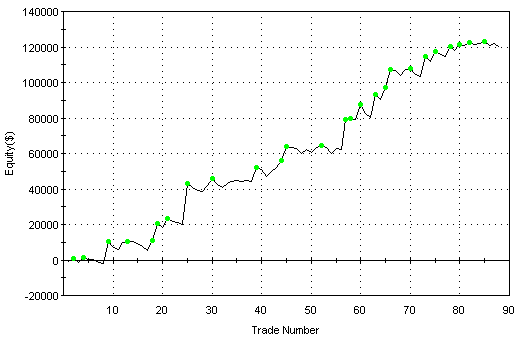
Figure 1. One-contract equity curve for the system optimized on US T-bonds over 12/29/1980 to 12/29/2000. $75 was deducted from each trade for slippage and commissions.

The optimized results were as follows:

Net Profit: $119963

Number of trades: 88

Percent Profitable: 45%

Average Trade: $1363

Profit Factor: 2.52

Max Drawdown: $18856

Testing the system on the out-of-sample period (12/30/2000 - 3/2/2005) produced the following results:

Net Profit: $12181

Number of trades: 18

Percent Profitable: 56%

Average Trade: $677

Profit Factor: 1.58

Max Drawdown: $17113

On an annualized basis, the net profit in the out-of-sample period is about half that in the optimized segment. The worst-case drawdown is about the same, and the percentage of profitable trades is slightly better.

Keep in mind that a very basic set of entry conditions was chosen, and there are no separate exit conditions. Better results could no doubt be achieved by improving both the entry and exit conditions.

To show how the results can differ depending on the market, I applied the same system to Live Cattle (symbol @LC.P, daily bars, in TradeStation 8). I optimized the seven weights over 15 years of data, 3/3/1986 to 3/2/2001, saving the latter years for out-of-sample testing. In this case, the set of weights that maximized the objective function produced too few trades for statistical significance, so I chose the weights that maximized the weighted net profit as calculated by the EqtyCorr3 function. This set of weights was as follows:

w1 = 1

w2 = 0

w3 = 1

w4 = 0

w5 = -1

w6 = -1

w7 = 0.

Only one of these weights is the same as for the T-bond example. This set of weights means long trades are entered when the following conditions are true:

C >= C[1] and C >= C[5] and C <= Average(C, 5) and C <= Average(C, 25).

This is a little harder to interpret than the conditions for T-bonds, but it looks like long trades are entered when the short-term trend is up and the longer-term trend is down -- a kind of mean-reverting logic. Again, the entry conditions for short trades are the logical opposite. The equity curve for the optimized system is shown below in Fig. 2.

Figure 2. One-contract equity curve for the system optimized on Live Cattle over 3/3/1986 to 3/2/2001. $75 was deducted from each trade for slippage and commissions.

The optimized results were as follows:

Net Profit: $30185

Number of trades: 37

Percent Profitable: 68%

Average Trade: $816

Profit Factor: 2.78

Max Drawdown: $7994

Testing the system on the out-of-sample period (3/2/2001 - 3/3/2005) produced the following results:

Net Profit: $18270

Number of trades: 6

Percent Profitable: 67%

Average Trade: $3045

Profit Factor: 6.10

Max Drawdown: $9510

On an annualized basis, the net profit in the out-of-sample period is actually about twice that in the optimized segment, although the worst-case drawdown is larger, and there are only six trades, so it's difficult to draw conclusions.

I did one more test to explore a different set of conditions. The conditions in the first two examples were simple momentum and trend conditions. The following conditions include five conditions that represent price pattern relationships plus two trend conditions:

C1 = C - C[1]

C2 = C - L[1]

C3 = C - H[1]

C4 = H - H[1]
C5 = L - L[1]

C6 = C - Average(C, 5)
C7 = Average(C, 5) - Average(C, 25)

where C is the close, L is the low of the bar, and H is the high of the bar. C7 is slightly different than before in that it represents the relative position of two moving averages rather than the position of the close relative to a moving average. For this test, I added the following exit condition: exit any open trade three days after entry.

I tested this version of the system on US T-bonds again. I optimized the weights over 12/29/1980 to 12/29/2000, saving the latter years for out-of-sample testing, as before. The weights that maximized the objective function defined by EqtyCorr3 were as follows:

w1 = -1

w2 = 1

w3 = -1

w4 = 0

w5 = -1

w6 = -1

w7 = 0.

This means long trades are entered when the following conditions are true:

C <= C[1] and C >= L[1] and C <= H[1] and L <= L[1] and C <= Average(C, 5)

On a chart, the first four conditions represent a fairly simple price pattern with a lower close and lower low, where the close is between the high and low of the prior bar. The last condition says that in addition to this price pattern, the short-term trend should be down. Trades are exited three days after entry. Interestingly, there are no short trades with these conditions. This is because if you reverse the equality signs on the first two conditions, they contradict each other; the close can't be above the prior close and below the prior low at the same time. With this set of conditions, changing the weight from +1 to -1 does not produce the logically opposite conditions. (To produce the logical opposite would require changing lows to highs and highs to lows.) This violates one of the assumptions stated at the outset but still produces meaningful results.

The equity curve for the optimized system in this case is shown below in Fig. 3.

Figure 3. One-contract equity curve for the modified system optimized on US T-bonds over 12/29/1980 to 12/29/2000. $75 was deducted from each trade for slippage and commissions.

The optimized results were as follows:

Net Profit: $47738

Number of trades: 286

Percent Profitable: 50%

Average Trade: $167

Profit Factor: 1.53

Max Drawdown: $7625

Testing the system on the out-of-sample period (12/30/2000 - 3/3/2005) produced the following results:

Net Profit: $10994

Number of trades: 63

Percent Profitable: 56%

Average Trade: $175

Profit Factor: 1.38

Max Drawdown: $6988

On an annualized basis, the net profit in the out-of-sample period is slightly greater than that in the optimized segment. The profit factor is not quite as high, but the worst-case drawdown is slightly lower, and the percentage of profitable trades is higher.

This rapid prototyping method can produce interesting results. The difference in results between the first version of the system applied to T-bonds and the same system applied to Live Cattle shows how different markets may require very different trading logic. Using this approach may be a good way to answer basic questions about a market you're studying, such as "Is it better to go long when the trend is up (e.g., buy breakouts) or buy on dips?" This is one of the advantages of this approach as compared with neural networks: the rapid prototyping approach produces a set of logical conditions that are easy to interpret.

I used a fairly simple set of conditions in the examples presented here. There's no reason why more complex or interesting conditions couldn't be applied, such as stochastics and Bollinger bands. However, to program an indicator like stochastics so that a weight value of +1 means to buy below a value of 20, for example, while a weight value of -1 means to sell above a value of 80 requires a little extra work.

Of course, there are limitations to the rapid prototyping method. Not all entry conditions fit within the framework outlined here. For example, if you want to test a day-of-the-week filter (e.g., buy on Mondays), there's no easy way to express that as an inequality. Even the last example didn't exactly fit the framework in that reversing the sign of the weight didn't produce the logically opposite condition. However, in that case, sell signals could be studied separately in a different system that only sold short.

As with any method that involves optimizing system parameter values, it's important to perform out-of-sample testing. As I've discussed in previous issues (see May 2003 issue), the more trades present in the optimization segment, the greater the likelihood that the results will hold up in both out-of-sample and real-time trading. Nonetheless, if used properly, the rapid prototyping approach might be a useful tool to aid in the process of trading system development.

That's all for now. Good luck with your trading.